Every machine learning project, no matter how sophisticated, rests on a handful of foundational ideas. In this post we build them from scratch using the UCI Adult Census Income dataset, a classic binary classification task where we predict whether someone earns more than $50,000 per year. By the time we finish, we'll have a working model that reaches 84 percent accuracy, and more importantly, we'll understand why it works and where it fails.
The dataset and what we found #
The Adult dataset contains 32,561 rows after removing duplicates and the fnlwgt
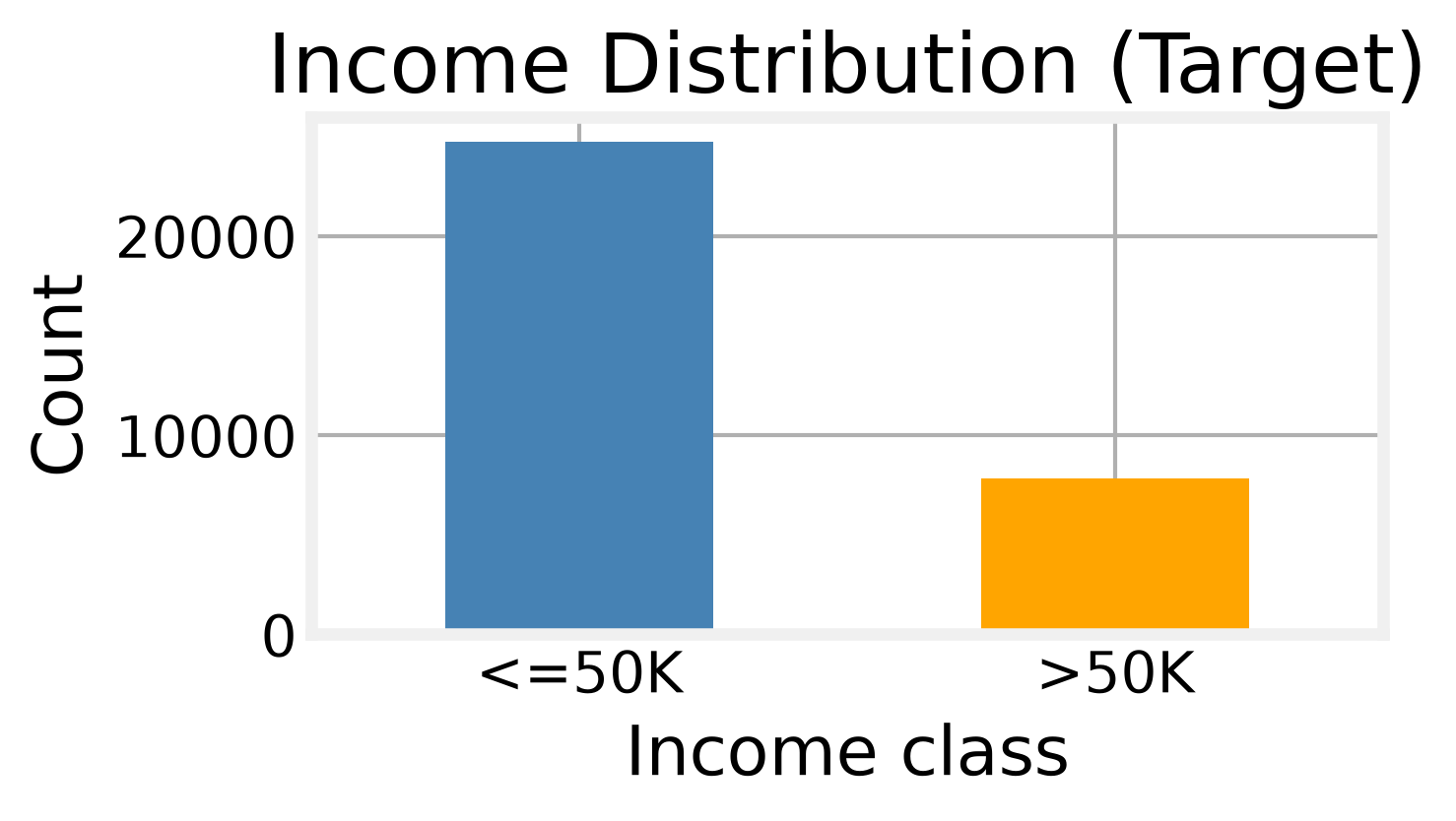
sampling weight column. Each row describes a person through 14 features: age, education, occupation, hours worked per week, and others. The target is imbalanced—about 76 percent of people earn $50,000 or less, and 24 percent earn more. That imbalance matters immediately: if we always predict the majority class, we achieve 76 percent accuracy without learning anything. That number is our floor.
We inspected the numeric features first. Age, education level, capital gains, capital losses, and hours per week all show reasonable distributions, though capital_gain
has a long tail. The correlation heatmap confirmed what we expected: no pair of numeric features is strongly correlated, so we won't need to worry about multicollinearity in our simple models.
The target distribution tells the story of the challenge ahead. A model that learns nothing beats three out of four predictions. To be useful, we need to beat that baseline. Now we tackle the first obstacle to beating that baseline: the risk of overfitting.
Overfitting #
A model that memorizes noise rather than signal is said to overfit. Let's see what that means. Overfitting is what happens when a model memorizes the training data instead of learning the underlying pattern. It scores high on the data it saw and low on data it hasn't. We demonstrate this with a deep decision tree.
deep_tree = DecisionTreeClassifier(max_depth=15, random_state=SEED)
deep_tree.fit(X_train, y_train)

train_acc = accuracy_score(y_train, deep_tree.predict(X_train))
test_acc = accuracy_score(y_test, deep_tree.predict(X_test))
The tree reaches 85.8 percent on the training set but only 83.8 percent on the test set. That gap of two percentage points is the signature of overfitting. The model has learned quirks of the training data—specific combinations of age and capital gain that happen to correlate with income in the sample but not in the population. The deeper the tree, the more it chases noise.
Underfitting #
If overfitting is one extreme, underfitting is the other. Underfitting is the opposite problem: the model is too simple to capture even the broad pattern. A tree with max_depth=1
(a single decision stump) shows this clearly.
shallow_tree = DecisionTreeClassifier(max_depth=1, random_state=SEED)
shallow_tree.fit(X_train, y_train)
train_acc = accuracy_score(y_train, shallow_tree.predict(X_train))
test_acc = accuracy_score(y_test, shallow_tree.predict(X_test))
This stump scores 80.2 percent on training and 80.5 percent on test. Both numbers are barely above the 76 percent baseline. The model learned one rule—probably something about education or hours worked—and stopped. It never saw the richer interactions that separate high earners from low earners. The gap between train and test is small, but both are low. That is underfitting.