In the background posts we built the pieces: tensors and automatic differentiation in Posts 2 to 5, and in Post 18 the MNIST dataset, its , and a first baseline model. This post puts those pieces under load. We build a multilayer perceptron on raw pixels, check a hand-derived gradient against autograd, then run a controlled sweep over seven activations, four initializations, three normalizations, and three regularizers, all on the same task. The through-line for everything below is a single idea: depth is a chain of multiplications, and every design choice in this post is a way of keeping the factors in that chain near one.
Data and scaling #
The factors in that chain start with the input scale, so we inspect the raw pixels before any transform. The dataset is MNIST, 70,000 grayscale images of 28 by 28 pixels, about 11 MB compressed. We keep the budget small on purpose, 10,000 train rows, 2,000 validation, 2,000 test, and a 4,000 row sweep slice, because the subject is the mechanics of depth and not the dataset. A full training run finishes in under a second on a CPU, which is what pays for a dozen short experiments instead of one long one.
We inspect the raw uint8 arrays before any transform, because transforms hide faults. Every pixel is present, there are no blank images, and no label falls outside 0 to 9. The label mix is near uniform, with a majority class rate of 0.1124, so guessing the most common digit is worthless and plain accuracy is a readable metric. We also hash every image and find no exact duplicates inside train and no test rows whose bytes repeat a train image, so the test number stays honest.
The intensity statistics drive the scaling choice. The global pixel mean is 33.32 with a standard deviation of 78.57, and 80.88 percent of pixels are exactly zero. The images are background dominated, so raw 0-to-255 inputs would push the first layer weights to tiny scales. We divide by 255 and flatten each image to 784 values.
Checking the class balance and pixel distribution shows what the scaling must fix.
The histogram is a spike at zero with a thin tail, matching the 80.88 percent zero-pixel count.
One more finding matters for the error floor. Ink per image ranges from 32 to 342 pixels, and a handful of faint samples carry almost no signal.
The faintest sample has 32 ink pixels; these low-signal rows set a floor that the best model in this post cannot cross. Perfect accuracy is not reachable here, and a small error floor is expected. Input dimension 784 and output dimension 10 now fix the shape of every model below.
Networks and backprop #
A multilayer perceptron stacks affine maps (a linear transform plus a bias) and nonlinearities. Two weight matrices are already enough to carve a curved boundary in pixel space. Training needs the gradient of one scalar loss with respect to every weight, and backpropagation produces it by walking the computational graph backward once. The whole story in one line: h = act(W1 x + b1), logits = W2 h + b2.
Forward-mode automatic differentiation carries a directional derivative forward and costs one pass per input. Reverse-mode automatic differentiation carries a cotangent backward and costs one pass per output. A loss is one scalar, so reverse mode is what trains neural networks. The universal approximation theorem says a wide enough single hidden layer can approximate any continuous function on a compact set. It says nothing about how hard those weights are to find, which is the subject of the rest of this post.
The first check is that autograd agrees with the chain rule by hand. We build a small graph, call backward, then compute the last-layer gradient manually as 2 times the logits divided by the number of elements.
h = torch.tanh(Xg @ W1 + b1)
logits = h @ W2 + b2
loss = (logits ** 2).mean()
loss.backward()

with torch.no_grad():
    dlogits = 2 * logits / logits.numel()
    manual_W2 = h.T @ dlogits
assert torch.allclose(manual_W2, W2.grad, atol=1e-6)
The maximum absolute difference between the manual and autograd gradients for W2 and b2 is 0.0, and walking the recorded graph shows a chain of named operations, MeanBackward0, PowBackward0, AddBackward0, not a black box. To see why reverse mode is the right choice, we implement forward mode with a small dual number class and compare the two on the same three-input function.
grad_fwd = [f_dual([Dual(point[j], 1.0 if j == i else 0.0) for j in range(3)]).d for i in range(3)]

xt = torch.tensor(point, requires_grad=True)
f_torch(xt).backward()
assert np.allclose(grad_fwd, xt.grad.numpy(), atol=1e-6)
Both modes return the same gradient, 0.367202, -0.40923, -0.377817, but the cost differs. Forward mode needs three passes for this function and would need 784 for our input dimension. Reverse mode needs one pass in both cases. That single column is why every framework trains with reverse mode.
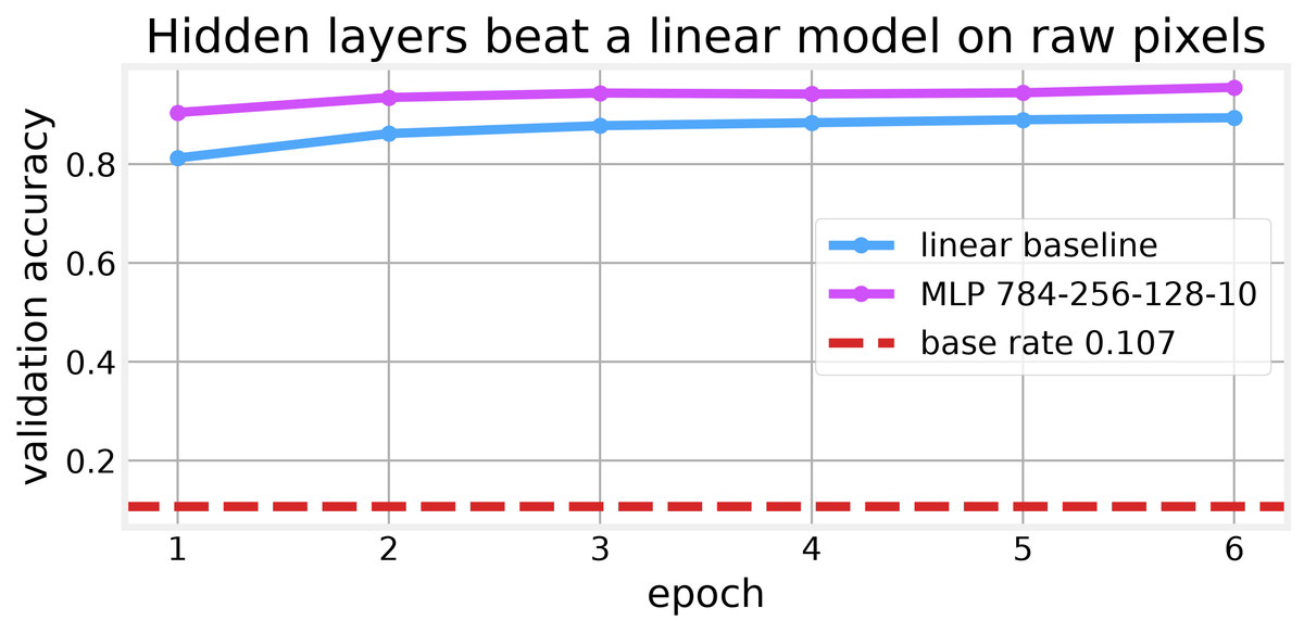
With the mechanics settled, we train two models. A linear softmax over 784 pixels lands at 0.8935 validation accuracy in 0.9 seconds, well above the 0.1074 base rate because digit classes are close to linearly separable in raw pixel space. An MLP with layers 784, 256, 128, 10 reaches 0.9550 in 0.8 seconds.