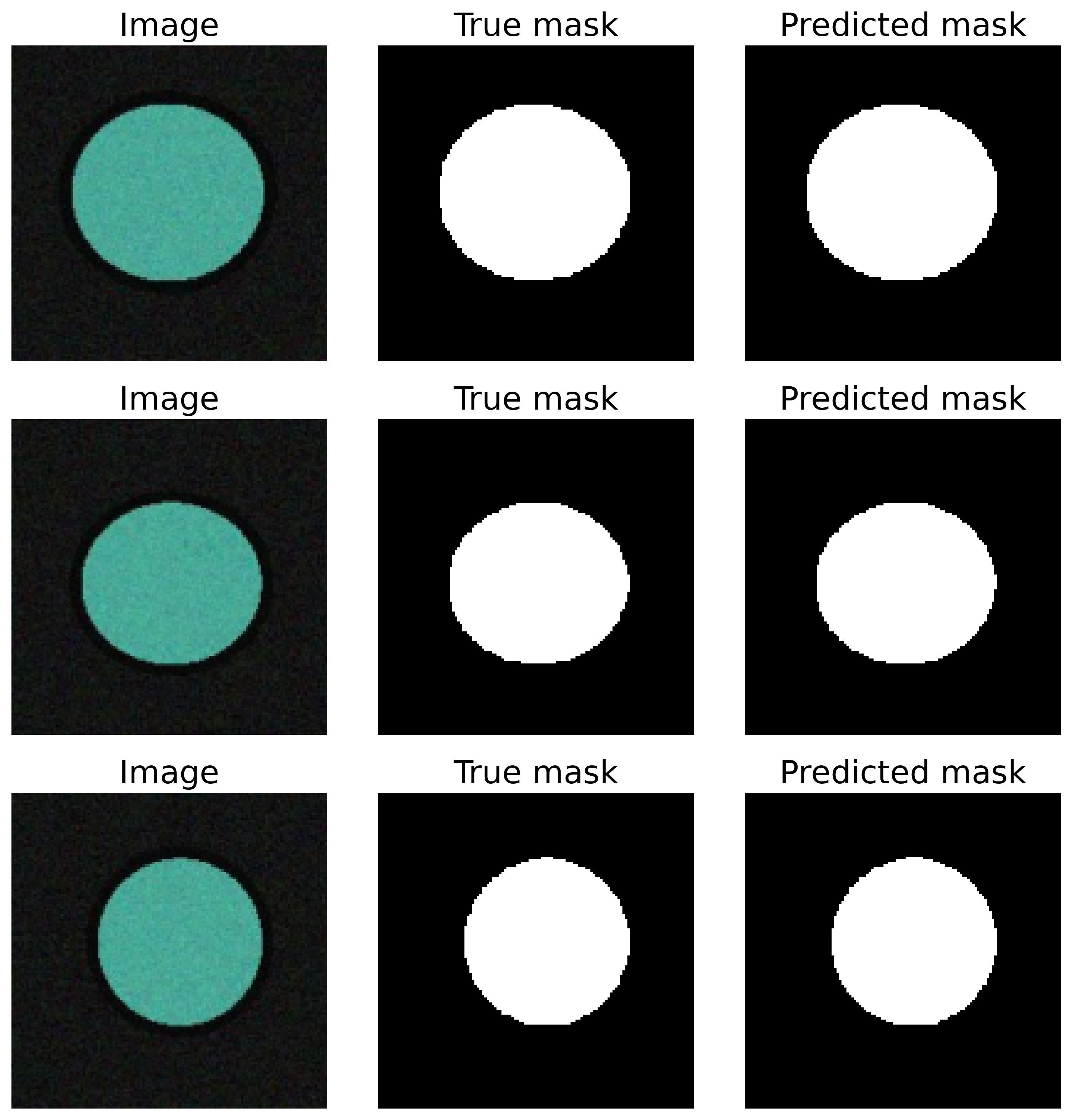
In the background posts we loaded and preprocessed image data, trained our first neural networks, and fine-tuned a pretrained backbone. Now we put all of that to work on a single dataset that asks two questions at once: which breed is this pet, and which pixels belong to the pet. By the end of this post we train a classifier that reaches 91.0 percent test accuracy on five pet breeds and a U-Net that paints a mask over the animal. The through-line we carry the whole way is the receptive field, the patch of input any single neuron can see. Every trick in this post is a way of growing, shrinking, or routing that patch.
We work with the Oxford-IIIT Pet dataset, 7,349 images of cats and dogs across 37 breeds, each with a pixel-level trimap mask. The notebook builds a small synthetic stand-in so the whole run finishes in minutes on a laptop, and the mechanics are identical to the real thing. We subsample five breeds to keep training short, which raises the random-guess baseline from 0.027 to 0.200, so we judge the model against the five-way baseline.
Looking before modeling #
Before any transform touches the data we inspect it raw, because transforms can hide faults. The synthetic frame has 5,180 rows and five columns: filename, breed, split, image_path, and mask_path. There are no missing values in the critical fields, no duplicate filenames, and no duplicate image content by a checksum of each file's first 1,000 bytes. The official trainval and test split has zero filename overlap, so we keep it and carve the trainval portion into train and validation.
A flat distribution makes 0.200 a fair chance baseline and keeps accuracy from hiding class imbalance. Every image is 160 by 160 with three channels, so resizing to 128 by 128 for modeling is a single uniform step. Pixel intensities span the full 0 to 255 range, so we normalize with ImageNet statistics for the pretrained classifier. We fix seed 42 for every split, initialization, and training run.
Convolution mechanics #
A convolution slides a small kernel over the image and sums the products, and the kernel learns to fire on edges, textures, and parts. The output size follows one formula: out = floor((in + 2·padding − dilation·(kernel−1) − 1) / stride) + 1, where dilation is the gap between kernel taps. Every knob we discuss is a term in that expression.
The first group of knobs controls spatial shape. Stride moves the kernel faster and shrinks the output, padding adds border pixels to keep the size, and max pooling keeps the strongest response in a window while average pooling keeps the mean. The second group controls channels and receptive field. Global pooling collapses each channel to a single number, and a 1x1 convolution mixes channels without looking at neighbors. Dilated convolutions skip pixels to grow the receptive field without extra parameters, and depthwise separable convolutions split a standard convolution into a depthwise pass and a pointwise pass to save parameters.
The cleanest way to see the mechanics is to run each one on a real image and read the shapes.
img_tensor = transforms.ToTensor()(img).unsqueeze(0).to(device)  # 1x1x128x128
conv_out = F.conv2d(img_tensor, kernel, padding=0)               # 126x126
conv_stride = F.conv2d(img_tensor, kernel, stride=2, padding=0)  # 63x63
conv_pad = F.conv2d(img_tensor, kernel, stride=1, padding=1)     # 128x128
A 3x3 kernel with no padding takes 128 down to 126. Stride 2 halves it to 63, and padding 1 restores it to 128. Max and average pooling both halve the spatial size to 64, and global pooling removes it entirely, returning a 1x1 map. A 1x1 convolution with four outputs carries only 8 parameters, which shows how cheap channel mixing can be. The depthwise separable block uses 18 parameters where the standard convolution needs 40 for the same channel change, because it splits the work into a depthwise pass and a pointwise pass.