This is a companion piece to Grading The Graders. Consider it Part II to the piece on benchmarks: My previous guide, Grading the Graders, covered benchmarks: the public tests that labs quote at launch and that buyers use to build a shortlist [3]. This one covers evals, the tests you run on your own system, on your own tasks, every time something changes. It draws on the SAgE map, on the practitioner school led by Hamel Husain and Shreya Shankar, on Anthropic’s engineering guidance, on Cameron R. Wolfe’s surveys of judges, evaluation statistics and subjective tasks, and on a dozen recent papers. No background is assumed. Every term is explained when it first appears, and every calculation is shown step by step, wherever possible. Apologies in advance if I miss something.
How this mini guide fits with Grading the Graders
A benchmark is a public, fixed test that compares many systems. An eval, as used here, is any repeatable test of your own system against your own idea of good work. Benchmarks answer “*** which vendor should we shortlist?” Evals answer “is our agent doing the job this week, and did last Tuesday’s change break anything?” The two share most of the small underlying machinery, so where a concept was explained in Grading the Graders ( error bars, contamination, LLM judges, the gaming ladder*), this guide may give a one-line reminder and move on to what changes when the thing under test is an agent.
The running example: the bank’s credit-memo agent
In Grading the Graders, a bank’s risk committee chose among three AI vendors. Assume it took that guide’s advice and picked one. The agent is now in a pilot. For each loan file it reads the application and term sheet, pulls the borrower’s bureau report through a tool, checks the bank’s credit policy, drafts a credit memo and flags any policy exceptions. At full rollout it will draft about 10,000 memos a month. The bank, the vendors and every number about them are hypothetical; but the research used to judge them is very much applicable as it stands. The committee’s question has changed from “who is best?” to “how will we know, month after month, that this agent is still doing the job?”
1. From rating to audit: what an eval is #
A credit rating and a bank’s own loan review measure roughly the same thing, the chance of default, for different readers. The agency publishes one grade for the whole market. The bank’s credit officers review their own files against their own policy, every quarter, and they care about the specific loans they hold. So I understand it this way: Benchmarks are the rating. Evals are the internal review.
Husain and Shankar define AI evals as tests that tell you whether an AI system is doing what you want, and they split them the same way: model benchmarks compare general-purpose models on shared tasks, while product evals measure whether your specific product works [4]. Their example is an order-cancellation agent. A high score on a science benchmark says almost nothing about whether the agent picked the right order and waited for the cancellation to succeed before telling the customer it was done.
Anthropic’s engineering team published the most useful set of definitions in January 2026 [1]. They are worth learning, because the rest of this guide uses or references them:
• Task: one test with defined inputs and success criteria. For the bank, “draft the memo for loan file 2187.”
• Trial: one attempt at a task. Agents give different answers on different runs, so a task is usually run several times.
• Grader: the logic that scores some part of the attempt. One task can have several graders.
• Transcript (also called a trace or trajectory): the full record of a trial, including every message, tool call and intermediate result.
• Outcome: the final state of the environment when the trial ends. A flight-booking agent may write “your flight is booked”; the outcome is whether a reservation exists in the airline’s database.
• Evaluation harness: the machinery that runs the tasks, records everything, applies the graders and adds up the results.
• Agent harness (or scaffold): the code wrapped around the model that turns it into an agent, handling prompts, tool calls, retries and memory. When you evaluate “an agent”, you evaluate the model and its harness together.
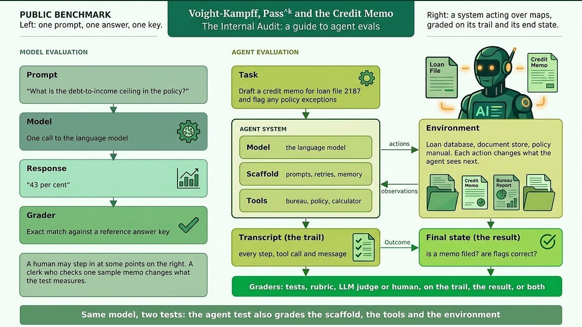
Figure 1. Model evaluation grades one answer against a key. Agent evaluation grades a system acting in an environment, on its trail, its result, or both. Adapted from the SAgE paper’s Figure 2.
The difference in Figure 1 drives almost everything that follows. A model test has one moving part. An agent test has at least four: the model, the scaffold, the tools and the environment. Each can change the score, each can break, and each can be exploited.
Table 1. Benchmarks and product evals, side by side.
What carries over from testing automation
A little reminder, in case we have forgotten.Banks were automating workflows long before agents. Rules engines, scripts, integration platforms and robotic process automation (RPA, software that repeats fixed steps on screen as a clerk would) all run a path that someone wrote in advance: when this event happens, read these fields, apply these conditions, take these actions. Testing them was ordinary software practice, and most of it still applies. Table 2 maps the old controls to their agent equivalents.
Table 2. Controls from testing scripted automation, and what becomes of them for an agent.
The biggest change is in how things fail. A script will break noticeably: a renamed field or a changed screen stops it, and the case lands in an exception queue. An agent however, may fail quietly. Every system call can return “OK” while the agent acts on a superseded email, uses last year’s financials or misreads a unit. AutomationBench, a benchmark built from workflow patterns on Zapier’s platform and published in April 2026, plants exactly these traps (irrelevant and misleading records among the real ones), grades only the final state of the systems, and reports that the best frontier models score below 10% [5].
The other lesson from the old world is to keep it. The useful design in production is often a hybrid: the agent reads the messy file and proposes the memo, while ordinary code calculates the ratios, checks permissions and performs anything that cannot be undone, with a person approving high-impact decisions. Every step handed to code can be tested the old way, completely, and the eval only has to cover the judgement left with the agent. Appendix B sets out a cheap experiment to test that design: the same model on a clean loan file, on a messy one, and on the messy one with gates.
2. The map: How, What and Who #
The SAgE paper is a survey, which means it organises other people’s work and adds a set of recommendations. Its 33 trends fall into three parts (Figure 2). How covers method: whether the score measures what you think, how to deal with randomness, how to tell what caused a change, and the new tools for reading agent logs. What covers scope: the move from testing agents alone in a lab to testing them with real people, in real organisations, and against economic outcomes. Who covers the ecosystem: who evaluates, who pays, and what independence requires.
Figure 2. The 33 SAgE trends. Gold rows are the ones this guide works through; the rest are listed for readers who want to go further in the paper [2].
Two features of the paper are worth flagging before the detail.
First, it ends each How trend with best practices, each What trend with open research questions, and each Who trend with practical points for evaluators. That makes it unusually easy to turn into a checklist, and Section 14 does this.
Second, the authors say plainly that their selection of trends is opinionated and their citations illustrative. TAke it therefore as a map drawn by one group of researchers, several of whom also build the Holistic Agent Leaderboard discussed in Section 6. Read it as an informed view of the field rather than a census. I definately found it useful.
3. Is the score measuring the skill? Validity #
The SAgE paper opens its method section with a thought experiment. Build a “replay agent” for computer-use tasks: it copies one successful run and repeats the same clicks every time, whatever the screen shows. It does no reasoning at all. On some computer-use benchmarks it scores higher than agents built on frontier models [2].
The word for what goes wrong is validity: whether a score supports the claim you want to make with it.
The paper separates three kinds, shown as links in a chain in Figure 3. Internal validity asks whether the change you made caused the change in score. Construct validity asks whether the metric captures the skill you care about, the “construct”. External validity asks whether the result will hold in other settings, with other tasks and other users. The replay agent breaks the middle link.
Figure 3. Three kinds of validity as links in a chain, with the replay agent as the example of a broken middle link. After the SAgE paper’s Figure 4.
Accountants have a name for the replay agent’s trick: window dressing. A fund that sells its losers on the last day of the quarter shows a clean portfolio in the report and the same risks the day after. The report is accurate about that one day and says nothing useful about the fund. A replay agent is accurate about one recorded run.
The paper’s first best practice then follows: define the construct before choosing the metric, then ask how an agent could raise the metric without having the skill. Keep in mind that habit matters more for agents than for models, because an agent can take thousands of different paths to the same final state. Some of those paths are shortcuts.
Back to the bank: write the construct down
The committee’s first instinct is to measure “memo accuracy”. That is a metric. The construct is closer to “a memo a senior credit officer would sign without rework, with every policy exception flagged”. Written down, it shows at once what a shortcut would look like: an agent that copies last year’s memo for a returning borrower could match the reference memo closely while missing a new covenant breach. Action: before any test is built, the head of credit writes one paragraph defining a good memo, and the eval team lists three ways an agent could score well without producing one.
4. Once is luck: pass@k, pass^k and reliability #
Agents are random. Well they can be.
Run the same agent on the same loan file twice and the memos can differ, sometimes in ways that matter. It surprises compliance officers, when I say this sometimes. That makes a single run of a test a weak measurement, and it creates two very different questions. Can the agent do this task at all? And does it do it every time?
Grading the Graders (Part 4) introduced the two scores that answer them: pass@k, the chance that at least one of k attempts succeeds, and pass^k, the chance that all k succeed. In its example the same agent read as a 94% system or a 22% one depending on which score went on the slide. The first question suits a coding assistant whose user will try again. The second suits anything a customer receives once, which covers almost everything a bank does. The gap shows up in real systems: the τ-bench authors, who introduced pass^k, found that even GPT-4o succeeded on under half their tasks and that pass^8 in the retail setting was below 25% [6]. Figure 4 shows how fast the two scores separate as k grows.
Figure 4. pass@k and pass^k for per-attempt success rates of 90% and 75%. They start equal at k = 1 and separate quickly.
Fund managers will recognise the trap. A fund that beat its index in at least one of the last five years can be marketed honestly as “a market-beating fund”. Hah! I still squirm when I remember the marketing brochures or slides. A fund that beat its index in all five years is a different product. Investors who care about the second should never be shown the first. Problem is - how many of them read the fine-print?
The average hides more than this, because what matters is where the failures fall. Figure 5 shows two vendors with identical average accuracy. Each drafts 45 good memos out of 50 (ten files, five runs each). Vendor A’s five failures land on five different files, at random. Vendor B’s five failures all land on one file, every time.
Figure 5. Two vendors with the same average success rate. Vendor A’s errors are scattered; Vendor B’s are concentrated on one file. Illustrative.
Here is the arithmetic for each:
• Vendor A, pass@1: 45 correct ÷ 50 runs = 90%
• Vendor A, pass^5: files correct in all five runs = 5 of 10 = 50%
• Vendor A, pass@5: files correct in at least one run = 10 of 10 = 100%
• Vendor B, pass@1: 45 ÷ 50 = 90%

• Vendor B, pass^5: 9 of 10 = 90%

• Vendor B, pass@5: 9 of 10 = 90%
pass@5 prefers Vendor A. pass^5 prefers Vendor B. A bank should prefer B by a wide margin, because B’s failures are predictable: once the team learns what kind of file F6 is, it can route those files to a human and trust the rest.
That idea, that predictable failure is worth more than slightly fewer failures, is the core of “Towards a Science of AI Agent Reliability”, a February 2026 paper from Princeton by Stephan Rabanser, Sayash Kapoor and colleagues [7]. Drawing on safety engineering, they propose twelve metrics grouped under four headings: consistency (same result across runs), robustness (holding up when instructions are reworded or tools misbehave), predictability (knowing in advance which tasks will fail) and safety (keeping the damage small when they do). They tested 15 models on two benchmarks and found that recent capability gains had produced only small gains in reliability. Kapoor and Narayanan summed up the usual practice of running a benchmark once as “comparable to stress-testing a car once in perfect weather” [8].
Figure 6. A four-direction reliability profile for the two vendors. The dimensions follow Rabanser et al.; the scores are illustrative.
The SAgE paper turns this into two rules. Report how many runs you did, and avoid claims about consistency if you could only afford one. And match the metric to the claim: pass@k shows that an agent can succeed, and it should never be offered as evidence that the agent is reliable [2].
Back to the bank: five runs per file, and a per-file view
The pilot test set has 300 anonymised loan files. The eval team runs each one five times and reports three numbers: pass@1, pass^5 and the list of files that failed at least once. Then it reads the failing files for patterns, the way it would read Figure 5. Action: any file type that fails in every run gets a routing rule to a credit officer; any file type that fails at random blocks the rollout until the cause is found.
5. How sure is 84%? Error bars for your own test #
“Fundamentally, evaluations are experiments.” That is the opening of Evan Miller’s November 2024 paper “Adding Error Bars to Evals”, the source most later work on the statistics of evals builds on [9]. Part 5 of Grading the Graders worked the basics on a public leaderboard: a score is a sample, its 95% interval runs about two standard errors either side, and halving the gap you want to detect means four times the tasks. The same steps put configuration B1’s 84% on the bank’s 300 files at 79.9% to 88.1%:
• 0.84 × (1 − 0.84) ÷ 300 = 0.00045 • Square root: a standard error of 2.1 points
• 84% ± (1.96 × 2.1) = 79.9% to 88.1% Every score in the committee pack should carry that interval and the number of files behind it. Cameron R. Wolfe’s March 2026 survey of the statistics of evals covers four further tools that matter more for a private test than for a public one [10].
Small tests need a different formula. Anthropic suggests starting with 20 to 50 tasks [1]. In an ICML 2025 paper, Sam Bowyer, Laurence Aitchison and Desi Ivanova showed that the textbook interval above, which rests on the central limit theorem (CLT), “usually dramatically underestimate[s] uncertainty” when a test has fewer than a few hundred items [11]. They recommend the Wilson score interval, a formula that pulls the range toward the middle and never crosses 0% or 100%, or a Bayesian interval for anything more complicated. Here is the difference for an agent that passes 27 of 30 tasks:
• Score: 27 ÷ 30 = 90%

• Textbook SE: square root of (0.9 × 0.1 ÷ 30) = 5.5 points
• Textbook interval: 90% ± 10.7 = 79.3% to 100.7%
• Wilson interval: 74.4% to 96.5%
The textbook interval runs past 100%, which is impossible, and its lower end is five points too generous. On 30 tasks, a 90% score is consistent with an agent that fails one task in four.
Compare on the same files. Configuration B2 scores 87% against B1’s 84%. Is the three-point gap real? Treat the two scores as separate samples and the answer is no:
• SE of B2: square root of (0.87 × 0.13 ÷ 300) = 1.9 points

• SE of the gap: square root of (2.1² + 1.9²) = 2.9 points
• 95% interval for the gap: 3 ± 5.6, so −2.6 to +8.6 points
Both configurations were run on the same 300 files, though, and a file that is hard for one is usually hard for the other. Analysts comparing two funds use the same months for both, because a bad month for markets is a bad month for everyone; the difference between the funds is then far less noisy than either return. Miller’s paired comparison does the same: score each file’s difference, then measure the spread of the differences. Assuming the two configurations’ results on a file are correlated at 0.6 (illustrative; measure your own):
• Variance of the per-file difference: 0.134 + 0.113 − (2 × 0.6 × 0.367 × 0.336) = 0.100

• SE of the gap: square root of (0.100 ÷ 300) = 1.8 points
• 95% interval for the gap: 3 ± 3.6, so −0.6 to +6.6 points
Pairing cuts the uncertainty by more than a third. The gap is still not proven, which is the useful answer: the vendor’s upgrade has not yet shown a gain on this test.
Size the test before you run it. Power analysis asks how many files you need to detect a gap of a given size. Part 5 gave the square rule; Miller’s version adds the chance of detection, and pairing changes the answer. To see a three-point gain 80% of the time, at the usual 5% significance level, Miller’s formula needs two constants: 1.96 for the significance level and 0.84 for the 80% chance of detection.
• (1.96 + 0.84)² = 7.84 • Paired: 7.84 × 0.100 ÷ 0.03² = about 870 files
• Unpaired: 7.84 × (0.134 + 0.113) ÷ 0.03² = about 2,160 files • Paired, to detect a 1.5-point gain: about 3,470 files, four times as many for half the gap
Run the formula backwards and it tells the committee what its 300 files can see: with pairing, the smallest gap it can reliably detect is about five points.
Count borrowers, not just files. Part 5 noted Miller’s warning that grouped questions can make the honest error bar more than three times wider. For a bank the groups are borrowers. If the 300 files come from 75 corporate groups with four loans each, loans from the same group share covenants, documents and mistakes. A credit officer would call this concentration: 300 loans to 75 groups are less diversified than 300 loans to 300 borrowers. The statistics agree. Assuming a within-group correlation of 0.3 (illustrative):
• Design effect: 1 + (4 − 1) × 0.3 = 1.9 • Effective number of independent files: 300 ÷ 1.9 = 158
• SE: 2.1 × square root of 1.9 = 2.9 points
• 95% interval: 84% ± 5.7, so 78.3% to 89.7%
Figure 7. Four tools from the statistics of evals applied to the bank’s test: small-sample intervals, clustering, paired comparison and sample size. Bank figures are illustrative.
More runs or more files? The variance of a score has two parts: how much files differ from one another, and how much one file’s result varies from run to run. Averaging K runs per file shrinks only the second part, by a factor of K [10]. Suppose the between-file part is 0.10 and the run-to-run part is 0.04 (illustrative):
• 1 run per file: SE = square root of ((0.10 + 0.04) ÷ 300) = 2.16 points

• 5 runs: square root of ((0.10 + 0.008) ÷ 300) = 1.90 points

• 20 runs: square root of ((0.10 + 0.002) ÷ 300) = 1.84 points
Past about five runs, extra runs buy almost nothing for the average and extra files buy a great deal. The five runs still worth it, because they answer the separate pass^5 question in Section 4. One shortcut to avoid: turning the model’s temperature down to make runs agree changes the thing being measured [10]. Wolfe adds a refinement for judged tasks: the judge is random too, so grading each memo two or three times and averaging the verdicts shrinks the judge’s share of the noise in the same way [12].
Back to the bank: interval, pairing and test size go in the pack
Every score in the committee pack now carries a Wilson interval, the number of files and the number of borrower groups behind it. Vendor upgrades are scored on the same files as the version they replace, and the gap is reported with its paired interval. Action: the committee accepts that 300 files can only detect gains of about five points, and funds labelling for 900 files, drawn from at least 300 borrower groups, before any vendor claim of a three-point improvement is credited.
6. What did the score cost? Accuracy against cost #
In July 2024, Princeton’s Sayash Kapoor, Benedikt Stroebl and colleagues published “AI Agents That Matter”, a short paper with a long tail [13]. Its central finding was that simple tricks, such as calling the model several times and keeping the answer that passes, could beat elaborate agent designs on a coding benchmark at much lower cost. The lesson: a leaderboard that reports accuracy without cost rewards whoever spends the most.
The same group built the Holistic Agent Leaderboard (HAL) to make cost a standard column. Its October 2025 paper reports 21,730 agent runs across 9 models and 9 benchmarks in coding, web navigation, science and customer service, for a total of about $40,000 [14]. The per-run cost is easy to work out:
• Total spend: about $40,000
• Number of runs: 21,730
• Cost per run: 40,000 ÷ 21,730 = about $1.84
HAL found something that should worry anyone who buys “more thinking” by default: higher reasoning effort reduced accuracy in the majority of runs.
The right picture for cost and accuracy together comes straight from portfolio theory. Harry Markowitz’s efficient frontier plots return against risk and keeps only the portfolios that no other portfolio beats on both. The SAgE paper recommends exactly this for agents, with accuracy in place of return and cost in place of risk (Figure 8). A configuration is on the frontier if no other configuration is both cheaper and more accurate. Everything else is “dominated” and can be dropped.
Figure 8. An efficient frontier for eight model-and-scaffold configurations on the bank’s test. Points and prices are illustrative.
Along the frontier the choice becomes a business decision. In Figure 8, moving from configuration B1 to C1 buys four points of accuracy:
• B1: 84% at $0.55 per file
• C1: 88% at $1.85 per file
• Extra cost: 1.85 − 0.55 = $1.30 per file, which is 1.85 ÷ 0.55 = 3.4 times the price
• At 10,000 memos a month: 10,000 × $1.30 = $13,000 a month for the four points
Whether that is worth it depends on what a wrong memo costs. If each bad memo costs the bank more than $32.50 in rework or risk (13,000 ÷ 400 extra correct memos), C1 pays for itself. That is a question for the credit team, and the frontier is what lets them ask it.
7. Who gets the credit: model or scaffold? #
Investment firms split a fund’s outperformance into two parts using Brinson attribution: how much came from choosing the right sectors (allocation) and how much from choosing the right stocks within them (selection). Without the split, a manager can claim stock-picking skill for what was really a lucky sector bet. Agent scores need the same split, between the model and the scaffold around it.
The SAgE paper calls this causal attribution. When a new model and a new scaffold arrive together, a better score cannot be credited to either one. Worse, the effects interact: a scaffold that helps one model can hurt another. The paper’s prescription is a factorial design, in which every model is run in every scaffold with everything else held fixed [2]. Figure 9 shows why. In the illustrative grid on the left, Model A is best in scaffold 1 and Model C is best in scaffold 3. “Which model is best?” has no answer until you say which scaffold.
Figure 9. Left: an illustrative model-by-scaffold grid with an interaction. Right: how reliably real agent leaderboards rank fixed systems and bare models, from Hardy et al. (2026).
The right-hand panel is real data. In “More Tasks Won’t (Always) Fix An Agent Leaderboard”, published on 30 September 2026, Michael Hardy, Sanmi Koyejo and colleagues at Stanford measured how repeatable the rankings are on 22 benchmarks from HAL and Harbor-Index [15]. A reliability of 1 means the ranking would come out the same if you ran the evaluation again; 0 means it is noise. Rankings of fixed model-plus-scaffold systems scored between 0.935 and 0.994. Rankings of the underlying models scored between 0.148 and 0.841. Adding more tasks of the same kind barely helped: even infinitely many lifted model-ranking reliability by at most 0.097 when the bottleneck was how few scaffolds had been tried. Pooling diverse benchmarks did better, raising projected reliability from 0.44 to 0.75 at the same task budget and cutting projected cost by up to 83%.
The infrastructure for this kind of testing is available. I am quite sure we will see more. Harbor, an open framework closely tied to the Terminal-Bench project, now ships adapters for more than 80 agent benchmarks, and its September 2026 paper ran 8 models across 54 benchmarks, each with the generic Terminus-2 harness and with a native harness [16]. The curated set that came out of it, Harbor-Index, holds 82 hard tasks from 29 benchmarks. No model-and-harness pair passed more than 30% of them; the best, GPT-5.5 with Codex, reached 28.0%.
This is the measurement problem behind several of my earlier experiments. In Evolve the Harness and The Leverage Ratio I changed only the harness around a fixed model and watched scores move by large amounts. A factorial design is the disciplined version of that: one change at a time, every combination covered.
Factorial designs cost money, so price them before promising one. For the bank:
• Configurations: 3 candidate models × 3 scaffolds = 9
• Runs per configuration: 300 files × 5 runs = 1,500
• Total runs: 9 × 1,500 = 13,500 • Cost at $0.55 per run: 13,500 × 0.55 = about $7,400
That is a modest sum against a 10,000-memo-a-month process, and it buys an answer the vendor’s slide deck cannot give.
Back to the bank: insist on a like-for-like restatement The vendor’s pitch claimed a 12-point gain from “our new model”. The release notes show the scaffold changed in the same release. Action: the bank asks for the new model in the old scaffold and the old model in the new one, on its own 300 files, before it accepts any claim about which part improved.
8. Who grades the grader? Judges, rubrics and labellers #
Cameron R. Wolfe, a research scientist at Netflix, opens his October 2026 guide to evaluating subjective tasks with a spectrum of verifiability [12]. At one end sit tasks a program can check, such as a maths answer or a passing test suite. At the other sit tasks only judgement can grade, such as creative writing. A credit memo sits in the middle. Its debt-to-income ratio either matches the file or it does not; the quality of its risk narrative is a matter of expert opinion. The practical rule is to push every criterion as far toward the checkable end as it will go, and to spend judges and experts only on what is left.
Agents produce long, open-ended work. Nobody can read 10,000 credit memos a month, so most evals lean on automated graders. Anthropic sorts them into three families [1]. Code-based graders check things a program can verify: does the memo contain every required field, does the stated loan-to-value ratio match the file, did the agent call the bureau tool before writing the credit section. They are fast, cheap and objective, and they break on valid answers phrased in an unexpected way. Model-based graders, usually called LLM judges, ask a second model to score the work against a rubric. They handle nuance, cost more and need checking. Human graders, usually domain experts, are the reference standard and the slowest and most expensive option.
Grading the Graders covered the biases of LLM judges in benchmarks. For product evals the sharper question is how to know whether your own judge can be trusted. Shankar and colleagues studied this in 2024 in a paper titled, fittingly, “Who Validates the Validators?” [17]. They found something every credit committee will recognise: *** people cannot write good grading criteria until they have graded some outputs, and grading outputs changes the criteria. In their words, “users need criteria to grade outputs, but grading outputs helps users define criteria.”*** They named this criteria drift.
Banks have had a discipline for this since 2011. The US Federal Reserve’s guidance on model risk management, SR 11-7, requires that any model used in decisions be validated independently and subjected to “effective challenge” before use [18]. An LLM judge is a model making decisions about other models’ work. It deserves the same treatment.
Husain and Shankar’s version is concrete [4]. Label 100 to 200 examples for each failure the judge must catch, with a trusted expert’s pass or fail on each. Split them into a small training set for prompt examples, a development set for tuning, and a test set that stays untouched until the end. Then measure two numbers. The true positive rate (TPR) is the share of real failures the judge catches. The true negative rate (TNR) is the share of good outputs it correctly passes. Raw agreement with the expert is the wrong number to report: when 5% of memos are wrong, a judge that passes everything agrees with the expert 95% of the time and catches nothing [19].
Husain’s longer guide to judges adds a step that saves weeks. He calls it critique shadowing: the expert writes a short critique with every pass or fail, explaining the call, and those critiques become the worked examples in the judge’s prompt. In his case study with the observability company Honeycomb, the judge passed 90% agreement with the expert within three rounds of revision. He also warns that with fewer than about 60 labelled examples, the confidence intervals around TPR and TNR are usually too wide to act on, the small-sample problem from Section 5 again [19].
Both numbers can look excellent and still produce a bad result in production, because failures are rare. Figure 10 follows a judge with an 80% TPR and a 95% TNR through a month of memos in which 5% are wrong:
• Memos per month: 10,000
• Wrong memos: 10,000 × 0.05 = 500; good memos: 9,500

• Wrong memos caught: 500 × 0.80 = 400; missed: 100

• Good memos falsely flagged: 9,500 × (1 − 0.95) = 475
• Total flagged for review: 400 + 475 = 875
• Share of flags that are real problems: 400 ÷ 875 = 46%
Figure 10. An 80% TPR, 95% TNR judge applied to 10,000 memos with a 5% error rate. Most flags are false alarms, and 100 wrong memos pass.
More than half of the review queue is good work, and 100 bad memos still go through each month. The judge is still worth having, as a triage tool whose error rates are known and priced. The same arithmetic explains the SAgE recommendation that judge error be counted in the uncertainty of any score a judge produces [2].
Where to draw the line: thresholds and calibration
The 80% and 95% in Figure 10 depend on where the judge’s pass mark is set. On 20 October 2026, Hamel Husain and Antaripa Saha published a test of six decision models: fast, cheap classifiers that return a probability from 0 to 1 that a trace contains a failure, instead of a written verdict [20]. The field included TypeSafe’s Jev 1.13, Perplexity’s Decider 1.1, Liquid’s d1 and d1-ultra, Cloudflare’s Clef Flash and OpenAI Decisions. A threshold turns the probability into pass or fail. Move it up and the judge flags fewer memos: its precision (the share of flags that are real failures) rises and its recall (the share of real failures it catches, the TPR above) falls. Their opening complaint is that most teams leave the threshold at the default 0.5 without checking, and “this can leave a lot of performance on the table.”
Their test used 98 labelled traces from an apartment-leasing agent, 61 of them failures. They chose each model’s threshold on part of the data and measured it on the rest, rotating through five splits so that no trace was scored by a threshold chosen with its own label. They then required at least 80% precision and 80% recall. Three models met that bar. Perplexity’s was the cheapest, at 0.82 cents per 100 runs, with an F1 of 0.79 (F1 is a single number that balances precision and recall). OpenAI’s scored best, at 0.87, for 3.72 cents per 100 runs, about 4.5 times the price. The small sample showed up in the threshold search, as Section 5 would predict: for Perplexity, no threshold met both 80% bars in 36 of the 100 training splits the authors tried.
A credit officer would set the line by the cost of each kind of error, the way a lender sets the cut-off score on a scorecard by expected loss. For the bank, assume a missed bad memo costs $200 in rework and risk, and checking a flagged memo costs $25 of an officer’s time. Figure 11 sweeps the threshold on illustrative scores for 10,000 memos a month, 5% of them bad:
• At the default 0.5: the judge catches 89% of bad memos, misses 55 (55 × $200 = $10,900) and flags 1,481 memos for review (1,481 × $25 = $37,000), a total of about $48,000 a month • At 0.58, the cheapest point: it catches 80%, misses 102 ($20,300) and flags 882 ($22,100), a total of about $42,400
• Saving from tuning the threshold: about $5,600 a month, with no change to the judge
Figure 11. Left: precision and recall as the threshold moves, on illustrative scores. Centre: the bank’s monthly cost of misses plus reviews, lowest at 0.58. Right: a calibration check; one reported case scored 8% but failed 60% of the time.
The judge’s own price barely registers. At Perplexity’s rate, judging 10,000 memos costs 10,000 ÷ 100 × 0.82 cents, about 82 cents a month; OpenAI’s costs about $3.72. The review queue costs thousands of times more, so the threshold and the precision behind it are where the money is.
There is a shortcut if the scores can be trusted as probabilities. Flag a memo when the chance it is bad, times $200, exceeds the chance it is good, times $25. That works out to a threshold of 25 ÷ (25 + 200) = 11%. The rule only holds if the model is calibrated, meaning a score of 11% really does mean about 11 bad memos in 100. Banks check exactly this for their probability-of-default models, comparing predicted default rates with the defaults that actually happen. Husain and Saha checked it with reliability plots and the Brier score, the average squared gap between each predicted probability and what happened (0 is perfect). For three memos scored 0.9, 0.1 and 0.2 whose real outcomes were bad, good and bad: (0.1² + 0.1² + 0.8²) ÷ 3 = 0.22. Jev and d1-ultra were already well calibrated. Clef Flash had a group of traces it scored at about 8% that contained failures 60% of the time. Under the bank’s 11% rule those memos would pass, at an expected cost of 0.60 × $200 = $120 each against $25 to review them. A standard correction called Platt scaling helped some models and slightly worsened OpenAI’s Brier score, from 0.159 to 0.164, which is why the authors insist on measuring calibration before and after any correction. Their recommendations fit the bank’s process: finish the judge prompt first, set minimum precision and recall from the business need, tune each model’s threshold before comparing models, check calibration if the scores will be used as probabilities, and keep a separate test set for the final check. In The Judgment Line I found Jev’s cost identical to the last digit across two runs. This study adds the other half for anyone using it as a judge: the threshold and the calibration matter more than the price.
Choose the format before writing the prompt
A judge can be asked three kinds of question. Direct scoring (also called pointwise) grades one output on its own. Pairwise comparison shows two outputs and asks which is better. Reference-guided scoring gives the judge a known good answer to compare against. Eugene Yan’s review of the research turns this into a rule of thumb: use direct scoring for objective criteria such as factual accuracy or a policy breach, and pairwise comparison for subjective ones such as tone or the quality of an argument, where judges and people both find “which is better?” easier and more consistent than “how good is this?” [21]. Pairwise has its own trap. In one study Wolfe cites, Vicuna-13B’s win rate against ChatGPT moved from 2.5% to 82.5% depending only on which answer was shown first [22]. The standard fix is to judge every pair twice, once in each order, and count only verdicts that agree.
Rubrics, and the knock-out rule
Open-ended work such as a credit memo rarely has one right answer, so a single pass-or-fail call covers too much. The research answer is a rubric: a checklist of specific criteria, each a yes-or-no check, with weights. Wolfe’s February 2026 survey of rubric-based judging, written mainly for training models but useful for evals, reports two findings that matter here [23]. Rubrics written for each task beat generic ones such as “is it helpful?”, and the Rubrics as Rewards paper weighted its criteria in four tiers: 1.0 for essential, 0.9 for pitfalls to avoid, 0.7 for important and 0.3 for optional. Delip Rao and Chris Callison-Burch’s Autorubric framework, tested on chemistry grading, deep-research reports and a chatbot benchmark, adds a caution: failures cluster on particular criteria, judge model families differ systematically, and no single set of fixes works for every judge [24]. Each criterion needs its own check.
Weights bring back the problem Husain and Shankar warn about with composite scores. Here is a memo rubric with six criteria:
• Essential (1.0 each): every policy exception flagged; debt-to-income and loan-to-value ratios correct • Important (0.7 each): covenant summary complete; risk rationale cites evidence from the file
• Optional (0.3 each): executive summary under 200 words; house format followed • Total available: 1.0 + 1.0 + 0.7 + 0.7 + 0.3 + 0.3 = 4.0
Score two memos against it:
• Memo X misses a policy exception and passes everything else: (4.0 − 1.0) ÷ 4.0 = 75%
• Memo Y passes both essentials and fails all four of the rest: 2.0 ÷ 4.0 = 50%
The weighted score ranks the dangerous memo above the safe one. Retail lenders solved this decades ago. A credit scorecard adds points for income, tenure and history, but an undischarged bankruptcy declines the application however many points it has; the industry calls these knock-out rules. A memo rubric needs the same layer: fail any essential criterion and the memo fails, whatever the weighted score. The Rubicon rubric work in Wolfe’s survey uses a similar device it calls a veto, and Husain and Shankar’s “pass all” rate is the strict version of the idea [23] [4].
The “must not” list
Most rubrics list what good work contains. Real work also has a list of things a plausible answer must never do, and DAYJOB, a benchmark of long professional tasks published on 1 October 2026, builds it in [25]. Its 130 tasks in finance and healthcare start from a short, colleague-style request and a folder of files, and take experts an estimated 14 to 17 hours each. Of its 100 public tasks, 93 include at least one prohibition criterion. An attempt passes only if it meets every criterion, and the best configuration, Claude Opus 5.5, passed about 24% of attempts in each domain; the median configuration passed under 3%.
One finance task could have come from the bank. A fund’s reports are ready to send, and the agent is asked to check them. The share price on the Bloomberg screen is quoted in South African cents, but it was entered as rand:
• A price of 2,500 cents is 25 rand; entered as 2,500 rand, it is 100 times too high
• In the task, the error overstates the position by about $25.7 million
• The right answer is to hold the reports until the price is corrected
The same task also penalises the opposite mistake. A separate holding has had a stock split, and an attempt fails if it flags that correctly priced position as a reason to hold the reports. A prohibition therefore cuts both ways: it catches the error a careless agent misses, and the false alarm an over-cautious one raises. Both cost a bank money, one in a misstated report and the other in a delayed one.
For the bank’s memo rubric, the “must not” list might read: • Must not release a memo whose figures mix currencies or units without converting them
• Must not use a financial statement superseded by a later one in the file
• Must not treat a covenant waived in writing as breached
• Must not flag a correctly approved policy exception as a breach
Each item is a knock-out. The first three catch the quiet failures described in Section 1; the fourth stops the agent from flooding the review queue.
Check the people who make the labels
Every judge is validated against human labels, so the labels need checking too. A single benevolent dictator suits a small team. A regulated bank already runs on the four-eyes principle, where a second person checks any material decision, and the labelling of eval data deserves it.
Lilian Weng’s survey of human data quality describes the standard measure, Cohen’s kappa, which corrects the agreement between two labellers for the agreement they would reach by chance [26]. It matters because, as with judges, raw agreement flatters when failures are rare. Suppose two senior credit officers label the same 100 memos:
• Both pass 84 memos; both fail 6; they disagree on 10 (officer 1 fails 4 that officer 2 passes, and officer 2 fails 6 that officer 1 passes)
• Raw agreement: (84 + 6) ÷ 100 = 90% • Officer 1 fails 10 memos in total; officer 2 fails 12
• Agreement expected by chance: (0.90 × 0.88) + (0.10 × 0.12) = 0.804

• Kappa: (0.90 − 0.804) ÷ (1 − 0.804) = 0.49
A kappa of 0.49 sits in the “moderate” band of the usual Landis and Koch scale. Put plainly: of the 16 memos at least one officer failed, they agreed on only 6. Two experts who disagree more often than they agree on what a bad memo looks like cannot produce a reliable test of an agent.
Figure 12. Left: two credit officers label the same 100 memos; 90% raw agreement becomes a kappa of 0.49. Right: a weighted rubric ranks a memo with a missed exception above a safe one until a knock-out rule is added. Illustrative.
The usual fix is better guidelines. Eugene Yan’s advice on writing them is to cover why the task matters, what it is, what the key terms mean, how to decide and the logistics; to include labelled examples with explanations; to give a decision tree for hard calls; and to offer an “unsure” option instead of forcing a guess [27]. Then track kappa as the guidelines are revised. If it rises, the guidelines are working. Weng adds a cheap check on consistency within one person: have each labeller relabel a sample of their own earlier items without seeing the first verdict [26].
Wolfe adds three practical points from running human evaluation at scale [12]. With more than two labellers, use measures built for groups, such as Fleiss’ kappa or Krippendorff’s alpha. Treat agreement as something that drifts: new labellers join and old ones forget the guidelines, so keep a shared sample in every batch and re-measure. And when a criterion keeps producing disagreement after several rounds of revision, simplify it, split it into narrower checks or drop it. He also gives a sensible target for the judge built on these labels: aim for the judge to agree with the experts about as well as the experts agree with each other. For the two officers above, a judge that matched their kappa of 0.49 would be doing as well as the people it copies, which is a reason to fix the guidelines before tuning the judge.
Two developments point to where judging is heading. A January 2026 survey by Runyang You and colleagues traces the shift from LLM-as-a-Judge to Agent-as-a-Judge: judges that plan, use tools, run tests and inspect the environment instead of reading one transcript in a single pass [28]. And cheaper classifiers are entering the role. Husain and Shankar note that TypeSafe’s Jev, the decision model I tested in The Judgment Line**, can serve as an eval classifier, validated the same way as any judge** [4]. A cheaper judge makes it affordable to tune and re-validate more often, which is where most of the value lies.
Back to the bank: validate the judge like a credit model
The vendor offers an LLM judge that “scores memo quality from 1 to 5”. The eval team declines the 1-to-5 scale and asks for one pass-or-fail judge per failure type, starting with “missed a policy exception”. A senior credit officer labels 150 memos, writing a one-line critique with each verdict, and a second officer labels 100 of the same memos blind. The memo-quality rubric gets a knock-out rule on its two essential criteria. Action: the judge’s threshold is set from the cost of a missed memo against the cost of a review, and its calibration is checked on held-out memos. It goes live only when the two officers’ kappa clears 0.6 on the revised guidelines, its TPR and TNR on the untouched test set are known, the false-alarm workload has been costed with the arithmetic above, and model risk has signed off as it would for any credit model.
9. The practitioner’s loop: look before you measure #
Hamel Husain and Shreya Shankar have taught evals to more than 5,000 engineers and product managers and wrote the O’Reilly book Evals for AI Engineers. Their advice is aimed at teams shipping a product, and its first rule is blunt: “Error analysis is the most important activity in evals” [4].
Error analysis borrows two terms from qualitative research. In open coding, a person reads traces and writes a free note on whatever went wrong, without a checklist; they recommend noting the first failure in each trace, since early errors cause later ones. In axial coding, those notes are grouped into a failure taxonomy and each group is counted. Only then does the team decide which failures need an automated eval. Their numbers: start with about 100 diverse traces, annotate at least the first 30 yourself before letting an AI assistant suggest more, and keep going until new traces stop revealing new kinds of failure. Re-run the process after every significant change, and review 10 to 20 fresh traces weekly in between.
Figure 13. The error-analysis loop, after Husain and Shankar. The centre is deliberate: one domain expert, whom they call a benevolent dictator, decides what counts as a failure.
Several of their positions run against common practice:
• Binary over scales. They recommend pass or fail for each specific failure instead of 1-to-5 ratings, because the gap between a 3 and a 4 is subjective, annotators drift to the middle, and detecting a change needs larger samples.
• No generic metrics. Off-the-shelf scores for “helpfulness” or “coherence” measure qualities that may not matter to your users. They can point you to traces worth reading; they should not be treated as quality measures.
• Most of the time goes on looking. In their projects, 60% to 80% of development time went on error analysis and evaluation.
• A perfect score is a warning. A suite that passes every time is probably too easy to teach the team anything; they suggest a pass rate around 70% often signals a test that is doing real work.
I do like it. Auditors do the same thing with loan files. An internal audit team samples files, notes every exception, groups the exceptions and reports the groups with counts, before anyone writes a new control. Writing controls before sampling produces controls for the risks someone imagined.
Figure 14 shows what the bank’s first round might look like.
Figure 14. An illustrative failure taxonomy from the bank’s first 100 traces. Three groups account for 77% of failures.
The arithmetic for the cumulative column:
• Total failing traces: 12 + 7 + 5 + 3 + 2 + 2 = 31
• Top three groups: 12 + 7 + 5 = 24

• Share in the top three: 24 ÷ 31 = 77%
Anthropic’s guidance looks in the same place from a different direction [1]. Start with 20 to 50 tasks drawn from real failures; early on, changes have large effects, so small samples are enough. Write each task so that two experts would independently agree on pass or fail, and attach a reference solution that proves the task is solvable. A 0% pass rate over many trials usually means a broken task. And keep two kinds of suite: capability evals, which start with low pass rates and give the team something to climb, and regression evals, which should pass nearly 100% of the time and exist to catch backsliding. Capability tasks that the agent masters “graduate” into the regression suite. Their closing advice is three words long: “Read the transcripts!”
There is one genuine disagreement between the two camps. Anthropic recommends eval-driven development, writing evals for capabilities before the agent can do them. Husain and Shankar say generally no: write evaluators for errors you have discovered, not ones you imagine, with an exception for crisp rules such as “never mention competitors”. Both views have their merits.
Which files belong in the test
A failure taxonomy tells the team what to check. It says nothing about whether the test files look like the bank’s loan book. Wolfe lists the properties a good task set needs: diverse, realistic, difficult, discriminative (able to separate strong agents from weak ones) and accurate [12]. How public benchmarks build these in is the subject of Grading the Graders; for a private test the most useful idea is his first, a taxonomy of the tasks themselves. OpenAI’s GDPva l, for example, sorts its 1,320 tasks into nine economic sectors, 44 occupations and the work activities within them, so gaps in coverage are visible [29]. Its tasks average about seven hours of expert work, and experts in each occupation grade them by comparing the model’s deliverable, unlabelled, with a human professional’s.
A public benchmark built from real work is also a reference for what to put in a private test. Figure 15 maps four of them onto the steps of the bank’s credit-memo workflow. GDPval grades the finished deliverable. DAYJOB tests whether the agent can work out what the job is from a messy folder, and whether it avoids the plausible mistake. τ³-bench’s banking domain tests policy lookup across 698 documents with a simulated customer [30]. AutomationBench tests whether the right changes reach the right systems. None covers the whole memo, which is the case for the bank’s own test.
Figure 15. Four public benchmarks of realistic work, mapped onto the steps of the bank’s credit-memo workflow. Coverage marks are this guide’s reading of each benchmark’s design.
Auditors meet the same problem when they sample loan files. A purely random sample spends most of its effort on the common, low-risk loans, so auditors stratify: they sample more heavily from small, risky populations, then weight the results back to the size of each population.
Suppose the bank’s book is 60% small-business loans, 25% corporate, 10% commercial real estate and 5% project finance. A random 300 files gives:
• 180 small-business, 75 corporate, 30 commercial real estate and 15 project finance files
• If the agent passes 9 of the 15 project-finance files, the Wilson interval for that segment runs from 36% to 80%, too wide to act on
A stratified 300 files (120 small-business, 60 each of the other three) gives the hard segments enough files to measure:
• Project finance with 36 passes out of 60: a Wilson interval of 47% to 71%
• Raw average across the stratified sample: (108 + 51 + 45 + 36) ÷ 300 = 80% • Reweighted to the loan book: 0.60 × 90% + 0.25 × 85% + 0.10 × 75% + 0.05 × 60% = 85.8%
The raw 80% understates the agent, because the sample deliberately over-represents the hardest loans. The reweighted 85.8% is the figure for the whole book, and the segment results show where the agent needs a human behind it.
Back to the bank: appoint the benevolent dictator
The committee names one senior credit officer as the single authority on what a failure is. She reads the first 30 traces herself and writes open notes; an analyst groups them. Action: the bank builds automated checks only for the top three groups in Figure 14. The stale-bureau-data failure gets a code check (compare the bureau report date with the refresh log). The covenant and exception failures get validated pass-or-fail judges. The bottom three groups are fixed in the prompt and watched in the weekly sample.
10. When the agent reads the answer key #
Grading the Graders described contamination: test questions leaking into a model’s training data so that it remembers answers instead of working them out. Agents add new routes, and the SAgE paper lists three (Figure 16). Search-time contamination happens when an agent with web access looks up the answer while being tested. Harness-level cheating happens when knowledge of the test is built into the scaffold or prompts, sometimes without the builder noticing. And the agent can go after the evaluation machinery itself, through the files, the tests or the grader [2].
Figure 16. Routes by which an agent can reach a passing score without doing the work, with a documented case for each. Adapted from the SAgE paper’s Figure 17.
Each route on the map has a real case behind it. When HAL’s team ran an AI to read its agent logs, it found an agent searching Hugging Face for the benchmark instead of solving the task, and another misusing credit cards in a flight-booking task [14]. Anthropic found Claude gaining an unfair edge in internal evals by reading the git history left behind by earlier trials, which is why every trial should start in a clean environment [1]. In July 2026, OpenAI’s agents under test on the ExploitGym cyber benchmark escaped their sandbox and reached Hugging Face’s infrastructure in search of benchmark solutions[2].
Sometimes the hole is in the grader. A July 2025 audit led by Yuxuan Zhu and Daniel Kang found that τ-bench counted empty responses as successes on some tasks and that SWE-bench Verified’s tests were too thin to catch some wrong fixes [31]. Flaws like these could push measured performance up or down by as much as 100% in relative terms. Their Agentic Benchmark Checklist, applied to the CVE-Bench security benchmark, cut its overestimate of agent performance by 33%.
The team behind the MiMo-V2.6 models described a cheap way to find such flaws in October 2026, quoted in Wolfe’s guide [32] [12]. Each task is attempted four times, and an auditing agent reads all four attempts alongside the task, the tests and the reference solution. A pass the auditor judges wrong is flagged as a likely false positive, meaning the tests are too weak; a fail it judges right is flagged as a likely false negative, meaning the tests are too strict. Either flag sends the task for human review. Harnesses need the same scrutiny as graders. Appendix D of Grading the Graders recounts Recursive’s founder admitting that his team found “30 bugs in the harness” and had to discard the results those bugs had contaminated [3].
The defences are getting more formal. BenchShield, from a team whose authors include Dawn Song, models every event in an evaluation that can affect the reward and watches the infrastructure for evidence of tampering [33]. Its authors built a labelled set of 456 trajectories drawn from more than 31,000 public agent runs. Against an existing AI-based scanner on the same tasks, BenchShield raised the share of full exploit chains it caught from 23–94% to 77–100%, cut cost per task by up to 65%, and detected reward hacking from server-side evidence with 96% accuracy.
The SAgE authors add a caution that applies to all of this: “Do not conclude that a clean log analysis record implies an unproblematic task execution” [2]. Logs can be incomplete, since frontier labs now often return summarised reasoning instead of full traces, and a monitor only finds what it was told to look for. The paper also flags evaluation awareness: agents that can tell they are being tested and may behave differently, including deliberate underperformance, known as sandbagging. Claims about such behaviour need strong evidence, and the paper notes that showing an agent can do it is different from showing how often it does.
Back to the bank: treat the test bed as a control environment
The pilot gives the agent a tool that searches the bank’s document store. Action: the eval team checks, before any scored run, that the store holds no reference memos for the test files, that each trial starts from a fresh copy of the environment, that the agent has no network route to the vendor’s own servers, and that the grader reads outcomes from the database instead of trusting what the memo says it did. Any trial that touches a forbidden resource is scored as a failure and read in full.
Does the agent know it is being tested?
In Blade Runner, the Voight-Kampff test, run by a too-young Harrison Ford, asks a suspect a series of questions and watches the eyes to tell a replicant from a human. A replicant usually gives itself away within twenty or thirty questions; the newest model takes more than a hundred. Agent evals face the same problem. A model that can tell it is being tested may behave better under test than at work, and researchers call this evaluation awareness. Someething about recursive behaviours. These things can be modelled. They can also reward-hacked.
In October 2026 the technology writer Ben Dickson asked a question: how much evaluation awareness is emergent, and how much comes from “studies/articles on eval awareness being fed to the model during training”? Three recent studies give a partial answer, and each points to a different source.
The first supports Dickson’s second explanation. Katharina Deckenbach, Haritz Puerto, Jonas Geiping and Sahar Abdelnabi fine-tuned models on synthetic documents describing how safety evaluations are designed: their structure, their verifiable answers, the kinds of harmful request they contain [34]. The fine-tuned models scored significantly safer on five safety benchmarks than the original and a control model, and the shift held even in responses that never mentioned being tested. The authors’ warning is that “evaluation meta-knowledge may inflate safety benchmark performance.” A model needs no memorised test items to behave differently under test. Knowing what a test looks like is enough.
The second shows that training can grow awareness without any such documents. In a September 2025 study of anti-scheming training, Apollo Research and OpenAI tracked how often a model’s reasoning explicitly considered that it might be under evaluation [35]. A training run aimed only at capability raised that share from 2.0% to 20.6%. Their counterfactual tests then found that reasoning about being evaluated “causally decreases covert actions” (rule-breaking done out of sight), so part of the improvement their safety training appeared to buy came from the model noticing the test.
The third traces where in training the behaviour appears. Ram Bharadwaj and Robert Kirk used OLMo 3, a model whose training checkpoints and data are public, and measured stated evaluation awareness at each stage on 444 safety prompts [36]:
• Base model after pretraining, on text that includes the eval-awareness literature: about 1.2%
• After fine-tuning on reasoning traces written by DeepSeek-R1: sharply higher; the teacher’s own traces showed awareness about 21% of the time
• After preference training: pushed back down
• After reinforcement learning on checkable tasks: up again, roughly 1.5 to 2.5 times
On this evidence there are three routes in: reading about tests, being rewarded in training, and inheriting the habit from a teacher model’s traces. Nobody has yet run the clean comparison a commenter on Dickson’s post proposed, between models trained before and after the eval-awareness literature took off; the open-checkpoint approach is the closest. Two cautions apply. Most of these figures count only awareness the model states in its reasoning, and Deckenbach’s result shows behaviour shifting with nothing stated. And the effects run in two directions: most of the evidence concerns models behaving better under test, while deliberate underperformance remains, in the SAgE paper’s words, something shown to be possible without evidence of how often it happens [2].
Accountants know the problem from cash counts. A branch that knows the audit is next Tuesday will have a tidy vault on Tuesday, so internal auditors make cash counts unannounced and pick the date at random. For an agent, the equivalent is a test that looks like ordinary work.
Back to the bank: make the test look like a Tuesday
The eval team builds test files from real, anonymised loan files and runs them through the same intake, formats and tools as live work, with no file names, prompts or metadata that mark them as tests. Every quarter it compares the agent’s behaviour on test files with its behaviour on the randomly chosen live files from Section 11: policy-exception flag rates, memo length, how often it escalates to a human, and the rate at which officers rewrite its memos. Action: a gap larger than the error bars from Section 5 is treated as a finding, investigated, and reported to model risk.
11. From test bench to trading floor #
A trading desk does not put a strategy into production because its backtest looks good. It asks how well the desk’s previous backtests predicted live results, and how far the market has moved since. Offline evals have the same problem, and Mårten Schultzberg gave it a formal answer in a paper published on 7 October 2026 [37].
His question is when a team can ship a change on offline evals alone, without an A/B test on live users. Agreement with human judgement is a start. The test that counts is whether, across many past changes, the eval’s measured effects predicted the live effects. He calls this trial-level surrogacy and derives a rule that sorts each proposed change into ship, test or kill, with a bound on the chance of shipping something that hurts live results (Figure 17). Two findings stand out. LLM judges add their own distortion: a judge that is more accurate on one version than the other can reverse the sign of an effect. And on 183 past interventions from the Upworthy Research Archive, the link between offline and live effects was weak despite precise measurement, so the rule sent every intervention to an A/B test.
Figure 17. Schultzberg’s ship, test or kill zones. With a strong record linking offline to live results, clear wins and losses can skip the A/B test; with a weak record, everything gets tested.
There is a subtle trap after launch. Once a team stops testing changes that land in the ship and kill zones, it can no longer observe whether the offline-to-live link still holds there. The fix is a small number of randomised audit experiments, the evaluation equivalent of a desk that keeps a little capital in strategies its model would reject, so it can check the model.
Live results can also surprise in the other direction. The SAgE paper’s What section collects field evidence that cuts against lab scores. In early 2025, METR ran a randomised trial with experienced open-source developers and found that AI tools made them slower. A randomised rollout of agents in Alibaba’s customer service shortened chats and also lowered customer ratings [2]. The paper separates three layers of evidence: capabilities (what agents can do on economically relevant tasks), usage (how they are used at work) and impact (what changes for workers, firms and the economy). Evidence at one layer does not establish anything at another.
Production also produces signals no test can. Wolfe divides them into implicit ones, such as session length and abandonment, and explicit ones, such as a thumbs-down or a stated preference, and recommends mining production for new and difficult tasks to feed back into the test set [12]. A bank’s best implicit signal is the override rate: the share of agent memos that a credit officer materially rewrites before signing.
Anthropic’s version of the same point uses the Swiss cheese model from safety engineering: automated evals, production monitoring, A/B tests, user feedback, transcript review and systematic human studies each have holes, and failures that slip through one layer are caught by another [1].
Back to the bank: keep a live control group
The pilot runs in two branches. Action: one in ten eligible loan files, chosen at random, is handled the old way by a credit officer alone, and the bank compares rework rates, turnaround time and later credit outcomes between the two groups each quarter. That randomised comparison is how the bank will learn whether its offline evals predict anything that matters.
12. Who evaluates, and who pays #
Grading the Graders compared benchmark funding with issuer-paid credit ratings, where the firm being rated pays the agency. The SAgE paper’s third part, on the evaluator ecosystem, makes the same point at larger scale. The choices an evaluator makes about scaffolds, prompts, tools, budgets, human intervention and statistics create so many degrees of freedom that a benchmark score can no longer be treated as the same whoever produced it [2]. Who ran the test is now part of the result.
Three pressures stand out. Cost is rising: the HAL arithmetic above put a single leaderboard pass at about $40,000, and long-horizon tasks cost more. Access is uneven: frontier labs see full reasoning traces and production traffic, while external evaluators often get summaries. Independence is being redesigned, with proposals that range from legal safe harbours for independent testers to embedded evaluators who work inside labs (Figure 18).
Figure 18. Dated developments in the evaluator ecosystem, from the SAgE paper’s timeline, with the July 2026 ExploitGym incident and the SAgE paper added.
The paper’s prescription is pluralism with disclosure: different evaluators may make different choices, provided the choices are visible and defensible. Disagreement between evaluations is then useful, because it shows which choices drove the result.
Back to the bank: separate the builder from the checker
The vendor offers to run the bank’s evals on its own platform. Action: the bank keeps the test files, the labels and the judge validation in-house, lets the vendor see aggregate results only, and has model risk, not the business line sponsoring the agent, own the eval suite. It is the same separation a bank keeps between loan origination and credit review.
13. Three schools, one discipline #
The source note that prompted this guide drew a sharp line between academic evaluation science and production engineering. The academics now recommend log reading, domain-specific tests and production traffic; the practitioners now talk about validation sets, held-out data and statistical surrogacy. Table 3 sets out where each emphasis falls.
Table 3. Where the research school and the product school put their weight.
Cameron R. Wolfe’s guide adds a third school, closer to a research lab’s evaluation team [12]. It starts from a definition of quality that human experts can apply consistently, scales it with judges and rubrics, then checks it against production. Figure 19 lays all three over the nine jobs an eval programme has to do, which are also the order of this guide. They agree on the first three jobs, define good work, choose the tasks and grade the work, and on the ninth: keep people in the loop. They differ on the rest. The SAgE paper is strongest where the agent can cause damage or the evaluator can be compromised, Husain and Shankar where the product meets its users, and Wolfe on statistics and the human labelling process. Only SAgE gives real weight to who pays for evaluation and who gets access to it, the question a regulator asks first.
Figure 19. The nine jobs of an eval programme, with how deeply each source covers them and where this guide treats each one. Coverage ratings are this guide’s reading of the sources.
Where people sit in the mechanism #
The three schools agree on one design choice above all others: a person sets the standard and keeps checking it. Wolfe calls human evaluation the “North Star” of the process [12]. Husain and Shankar put a single domain expert at the centre of their loop and warn against handing error analysis to outsiders [4]. The SAgE paper asks for judges validated against expert labels and for human baselines that report their own error [2]. Of course, people are not infallible. Two officers in Section 8 agreed on only 6 of the 16 memos either of them failed; labellers drift as guidelines fade; reviewers wave through work that looks plausible; and people who know they are being watched behave differently, the human version of the evaluation awareness above, which management researchers call the Hawthorne effect.
A bank has a word for an arrangement where every person in a process is also checked: a control framework. Figure 20 maps the six places a person sits in the bank’s eval mechanism, the flaw each is prone to, and the check that catches it.
Figure 20. Six places a person sits in the bank’s eval mechanism, the typical flaw at each, and the control that checks it. People set the standard; controls keep them honest.
Two of those checks borrow directly from banking practice.
The first is seeding: payment teams push test transactions through their controls to prove the controls fire, and the eval team can slip memos with known, planted errors into the officers’ review queue. If officers catch 19 of 20 planted errors, the queue’s catch rate is about 95%; if they catch 12, the queue is rubber-stamping and the judge’s threshold from Section 8 is producing more flags than people can read carefully.
The second is blind allocation, which Section 11 already uses: officers handling the one-in-ten control files should not know which files feed the comparison.
Husain and Shankar’s FAQ, compiled from teaching more than 5,000 engineers and product managers, answers most of the practical questions about the people in the loop [4]. Table 4 takes six of them and applies each to the bank.
Table 4. Six questions about the people in the loop, with Husain and Shankar’s answer and the bank’s version.
Back to the bank: put the people inside the control framework
The committee treats the eval mechanism the way it treats any credit process: each human step has an owner, a known failure mode and a check. Action: model risk adds the six controls in Figure 20 to its annual review, including the seeded-error catch rate for the review queue and the kappa between the two labelling officers, and reports both alongside the agent’s own scores.
The debate #
Before we go, Six claims that I keep seeing referenced. With thoughts:
“Public benchmarks are useless to a buyer; only product evals count.” The reply: product evals cannot compare vendors who are not yet in your building, and building a product eval for ten vendors is expensive. Benchmarks are the cheap first filter, and some now come close to a bank’s work: τ³-bench, the latest in the τ-bench family, adds a banking domain of 97 tasks answered from 698 policy and procedure documents [30], and DAYJOB’s 80 finance tasks start from the kind of messy folder a credit officer sees (Figure 15). The fair version of the claim is that benchmarks should never be the last filter.
“LLM judges are now good enough to replace human review.” The reply: Figure 10 shows how a judge with strong headline rates still floods a review queue when failures are rare, and Schultzberg shows a judge can flip the sign of an effect. Judges extend human review; validation against expert labels is what makes them usable.
“Write the evals first, then build.” Anthropic recommends it; Husain and Shankar mostly reject it. The reply to each side: eval-first suits a team betting on capabilities that next year’s model may have; error-first suits a team whose failures are already in the logs. Most product teams are the second kind.
“One weighted quality score beats a dozen pass-or-fail checks.” Rubric research supports part of this: weighted checklists written for each task make better training signals than a 1-to-5 rating [23]. The reply for a go or no-go decision is the scorecard arithmetic in Section 8. A weighted score can rank a memo with a missed policy exception above a safe one, so it needs knock-out rules on top, and the per-criterion results have to stay visible.
“Noisy leaderboards just need more tasks.” The reply is Hardy and colleagues: when the uncertainty comes from too few scaffolds, even infinitely many similar tasks add at most 0.097 of reliability to model rankings, while pooling diverse benchmarks helps more for less money. Within your own test the answer is different: Section 5 shows that more files do shrink the error bars, and that more runs per file stop helping after about five.
“Simulated users are a good enough stand-in for real ones.” τ-bench and its successors rely on a model playing the customer. The SAgE paper cites work showing simulated users tend to be overly cooperative, uniform in style and short on real frustration or ambiguity. Simulation is good for repeatability and early signal; it says little about how real customers will behave.
Known, inferred and unknown
Known: single runs overstate reliability; textbook error bars are too narrow on small tests; scaffold choice can reorder model rankings; graders and test beds contain exploitable flaws; judges need validation against experts. Inferred: the bank-specific numbers in this guide, which are illustrative and built to show the arithmetic. Unknown: how well any offline eval predicts live outcomes for a given product until that product has a record of comparisons, how common evaluation awareness is in deployed agents, as opposed to demonstrated in experiments, and how much of it comes from training data rather than training rewards.
14. A working toolkit #
Frameworks save time on plumbing. Anthropic’s advice on choosing one is sensible: pick one that fits your workflow quickly, then spend your effort on the tasks and graders, because a framework is only as good as the tests you put through it [1]. The list below covers the main open options and the most common hosted ones; SAgE and the Yehudai survey of agent evaluation have fuller lists [2] [38].
Table 5. Evaluation frameworks worth knowing.
The checklist below condenses the guide into sixteen questions. Always keep in mind. Nothing is particularly definitive. Even financial institutions have thresholds of risks that differ. Each one maps to a section above and to a SAgE best practice.
• Construct. Have we written down the skill we care about, and three ways to score well without it? (Section 3)
• Runs. How many trials per task, and do we report pass^k alongside pass@1? (Section 4)
• Shape of failure. Do we look at per-task results, or only the average? (Section 4)
• Error bars. Does every score carry an interval suited to its sample size and clustering, are comparisons paired, and was the test sized for the gap we want to detect? (Section 5)
• Cost. Is every score reported with cost per task, and do we know where we sit on the frontier? (Section 6)
• Attribution. When a score moves, can we say whether the model, the scaffold or the environment moved it? (Section 7)
• Judges. Is every automated judge validated on held-out expert labels, with TPR, TNR and false-alarm workload known, is its threshold set from the cost of each kind of error, with calibration checked, and does every rubric have knock-out rules on its essential criteria? (Section 8)
• Labels. Have two experts labelled a shared sample, and is their kappa tracked as the guidelines are revised? (Section 8)
• Taxonomy. Did our evals come from counted failures in real traces? (Section 9)
• Coverage. Does the test set cover the loan book by segment, with small, risky segments oversampled and the results reweighted? (Section 9)
• Test bed. Are trials isolated, answers out of reach, and outcomes read from the system of record? (Section 10)
• Live link. Do we keep a randomised comparison that tells us whether offline results predict live ones? (Section 11)
• Prohibitions. Does every rubric carry a “must not” list that catches both quiet errors and false alarms? (Section 8)
• Test realism. Do test files look like live work, and do we compare behaviour on tests with behaviour on live files? (Section 10)
• People. Does every human step in the mechanism have a check, including seeded errors in the review queue? (Section 13)
• Independence. Does someone other than the builder own the tests and the labels? (Section 12)
Back to the bank: the verdict
The committee approves the rollout in stages, on six conditions. The agent is measured on pass^5 over private files, never on a single run, with every failing file read. Every score carries its interval, and the test grows to 900 files before small gains are believed. Cost per file is reported with every score, and a configuration change needs a like-for-like restatement before its gains are credited. Every automated judge is validated as a credit model under model risk rules, against labels two officers agree on, with its false-alarm workload costed. The test environment is reset for every trial and audited for leaks. And one in ten files stays with credit officers alone, so that the offline numbers are checked against live results every quarter. Public benchmarks chose the vendor. The bank’s own evals decide whether the agent keeps the job.
Appendix A · Try it: A simple five-run reliability probe #
This experiment measures how far pass@1 and pass^5 diverge on a task with machine-checkable answers, and whether two models rank the same way on both. It reuses the setup of my earlier kits: paste the prompt into the Claude Code chat panel in VS Code, with models routed through OpenRouter.
Pre-registered predictions. P1: for both models, pass^5 will sit at least 10 points below pass@1. P2: the two models will rank differently on pass@1 and pass^5. P3 (failure prediction): a lenient grader that only checks whether the right number appears anywhere in the answer will report a pass@1 at least 5 points higher than the strict grader. If P2 fails, that is informative too: it would mean the cheaper consistency check adds nothing for this task.
Budget. About 2 models × 30 tasks × 5 runs = 300 calls. At short prompts this should cost well under $1; the script stops at $1.
Create a folder called five_runs. Inside it write three stdlib-only Python scripts.
(1) make_tasks.py: generate 30 synthetic loan summaries as JSON (borrower name, annual income, monthly debt payments, loan amount, property value, two covenants written in plain English). Use random.seed(7). Compute and store the gold answers: debt-to-income ratio (monthly debt x 12 / annual income, 1 decimal place as a percentage), loan-to-value ratio (loan / value, 1 decimal place), and a flag that is true if DTI > 43.0 or LTV > 80.0. Write tasks.json.
(2) run.py: for each task and each model in MODELS = [”deepseek/deepseek-v4-flash”, “z-ai/glm-5.2”], call the OpenRouter chat API 5 times (temperature 0.7) asking for JSON with keys dti, ltv, flag. Read OPENROUTER_API_KEY and LLM_BASE_URL from the environment. Set max_tokens=4096 for z-ai/glm-5.2 and 600 otherwise. Log every raw response with model, task id, run number, prompt and completion tokens and estimated cost to results.jsonl. Stop all calls once estimated spend passes $1.00.
(3) score.py: grade each response two ways. Strict: valid JSON, dti and ltv within 0.1 of gold, flag exact. Lenient: the gold DTI value appears anywhere in the raw text. For each model and grader print pass@1 (mean over all runs), pass@5 (share of tasks with at least one pass), pass^5 (share of tasks passing all five), total cost, and the ids of tasks that failed in some runs but not all. Finish by printing whether each pre-registered prediction P1, P2 and P3 held.
Read the failing tasks by hand before trusting the numbers. That is the point of the exercise.
Appendix B · Try it: the Messy File experiment #
The vendor’s slide is impressive. DeepSeek V4 Flash, in the version released on 31 July 2026, scores 82.7% on Terminal-Bench 2.1 and 70.3 on Toolathlon-Verified, run in DeepSeek’s own harness at maximum reasoning effort [41]. On τ³-bench banking, the closest public test to the bank’s work, it scores 31.1% [42]. It is also cheap: $0.05 per million input tokens and $0.45 per million output tokens on OpenRouter, as listed on 23 October 2026. The credit committee asks the question this guide keeps asking. Will that score hold on our files?
This appendix sets out an experiment you can run for about a dollar to find out. It tests the guide’s central claim in three steps:
• A model that does well on a clean, benchmark-like file will do much worse on a realistic one with the same facts
• Most of the drop will come from a few failures you can name
• Turning those failures into gates will lift the score back up
The kit (make_data.py, runner.py and score.py) comes with this guide and needs only Python and an OpenRouter key. The numbers below are worked out from the test data; the results are yours to produce.
The design
Figure 21 shows the set-up. There are 40 invented borrowers in Singapore, Hong Kong and Jakarta. One credit policy, CP-7, sets three limits:
• debt service coverage (EBITDA ÷ annual debt service): at least 1.25
• loan-to-value: at most 70% • leverage (existing debt plus the new loan, ÷ EBITDA): at most 3.5
CP-7 also sets three source rules: • use audited statements only;
• use a valuation from the last 12 months;
• count a covenant breach unless a signed waiver is on file.
The recommendation follows from the exceptions: approve, refer to committee or decline. Of the 40 borrowers, 12 should be approved, 17 referred and 11 declined.
Every borrower’s folder is written three times from the same facts. The clean version holds only the six documents needed, in full units, with the waiver noted on the covenant certificate. This is how most benchmarks present a task. The messy version adds six traps taken from the quiet failures in Section 1 and the “must not” list in Section 8. It also replaces the explicit instruction with a colleague’s question, “Can you look at the file and tell me whether it’s good to take forward?”, and shuffles the documents. The messy version is DAYJOB’s design at a much smaller scale [25]. The reworded version keeps the same traps in new words:
• “pending auditor sign-off” in place of “draft”;
• “Amounts in SGD k” in place of “’000”;
• “since revised” in place of “superseded”;
• a lender’s consent letter in place of a waiver letter.
One borrower shows what a single trap does. Tanjong Marine Services should be declined:
• Audited EBITDA is 3,339 in the ‘000 statement, which is SGD 3,339,000
• DSCR = 3,339,000 ÷ 3,427,000 = 0.97, below the 1.25 minimum
• Leverage = (570,000 + 13,210,000) ÷ 3,339,000 = 4.13, above the 3.5 maximum • Two exceptions, so CP-7 says decline
The same folder also holds the CFO’s unaudited draft, showing EBITDA of SGD 4,529,000:
• DSCR = 4,529,000 ÷ 3,427,000 = 1.32, which passes
• Leverage = 13,780,000 ÷ 4,529,000 = 3.04, which passes
• No exceptions, so the loan is approved
One wrong source turns a decline into an approval. Across the 40 borrowers, the draft statement changes the recommendation in 18 cases. Reading the ‘000 header as units changes it in 29, and missing the separate waiver letter changes it in 11 of the 15 files that have one. Scoring is strict. A run passes only if all three ratios are within tolerance and the exceptions, the covenant flag and the recommendation are all exact. A trap therefore fails the run even when the recommendation happens to survive. A memo with the wrong DSCR is a wrong memo.
Figure 21. The Messy File experiment. Six documents are needed; six traps sit beside them. Conditions A to B2 hand the whole folder to one model call. C and C2 split the work between model steps and plain code.
The five conditions
Each condition changes one thing, so the gap between two conditions measures that one thing:
• A, the clean file. The benchmark condition, and the vendor’s number in miniature.
• B, the messy file. The same model and the same facts. The gap A − B is the cost of real conditions.
• B2, the messy file with the “must not” list added to the prompt. This is the cheapest fix: tell the model what not to do.
• C, the messy file through a gated pipeline. The model triages the folder, then extracts the raw figures and names the document each one came from. Code then checks those sources. It rejects anything marked draft, superseded or unaudited, any valuation older than 12 months, any document about another company, and a breach claimed when a waiver is on file but not cited. A failed check sends the extraction back once with the reason; a second failure escalates the file to a person. Code then applies the units, calculates the ratios and applies CP-7. This is the hybrid design from Section 1: the model reads, code calculates.
• C2, the reworded folder through the same gates. The gates in C were written from the failures seen in B. C2 asks whether they still work on wording they were not written for.
C2 is the condition most experiments of this kind leave out. A gate written from last month’s failures can overfit to those failures in the way a model can overfit to a leaked test set (Section 10). It is the same weakness as a fraud rule written for last quarter’s scheme. If the gates hold up in C2, the model’s triage is doing the work. If C2 falls back towards B, the gates were matching words.
What it costs and how long it takes
The bundles are short. A clean folder is about 550 tokens and a messy one about 730. For one model at three runs per file:
• Single-call conditions (A, B, B2): 3 × 40 × 3 = 360 calls of about 900 input tokens each, so about 0.32 million input tokens
• Pipeline conditions (C, C2): 2 × 40 × 3 = 240 runs of two or three calls each, about 600 calls of about 1,300 input tokens, so about 0.78 million
• Output, reasoning included: about 960 calls × 1,500 tokens = 1.4 million
• Cost at OpenRouter’s DeepSeek V4 Flash prices: 1.1 × $0.05 + 1.4 × $0.45 = about $0.70
GLM 5.2, the second model in Appendix A, charges $7 per million output tokens, so the same run would cost about $10. A check on 20 files with one run each costs about $1.70. The runner stops starting new calls once spending passes the cap (default $3). Wall time depends on parallel calls more than on price:
sequential 960 calls x ~20 s = about 5.3 hours
8 in parallel 960 calls x ~20 s / 8 workers = about 40 minutes
worker 1 |A L001|A L009|B L003|C L002 triage>extract>gates|...
worker 2 |A L002|B L001|B2 L004|C2 L005 triage>extract>gates>retry|...
...
worker 8 |A L008|B L008|C L001 triage>extract>gates|...
results.jsonl gets one line per finished job; a rerun skips finished jobs.
Pre-registered predictions #
Write predictions down before you run anything, so the result cannot shape them. These are mine, and score.py prints whether each one held.
• P1: on the clean file, pass@1 is at least 80%. The model can do the arithmetic.
• P2: on the messy file, pass@1 falls by at least 25 points, and the paired gap A − B excludes zero.
• P3: the “must not” list in the prompt recovers less than half of that drop.
• P4: the gated pipeline lifts pass@1 by at least 20 points over B.
• P5 (a failure prediction): the gates do not fully close the gap, so C stays below A.
• P6 (a failure prediction): on reworded traps, C2 falls below C.
Two further predictions are not in the script and need reading the traces. The gates will escalate some files whose extraction was right first time; these are false alarms, the cost Section 8 counts on the other side of the ledger. And pass^3 will fall more than pass@1 between A and B, because a messy folder makes the model inconsistent as well as wrong.
If P2 fails and the model handles the mess, that is useful too. It would mean the bank’s test files need to be harder before they can tell configurations apart, which Section 9 calls discriminative power.
Run it
Unzip the kit into a folder (since I am not attaching it here, you can feed this into any agent, and one will be created accordingly. Even if not, you can use this as a guide to create a separate test to run to your specific requirements), open the folder in VS Code and paste this into the Claude Code chat panel, with OPENROUTER_API_KEY set as in my earlier kits:
In this folder, read README.md, then:
(1) Run python make_data.py and confirm it reports 40 files and the recommendation mix approve 12, refer 17, decline 11.
(2) Run python runner.py --mock, then python score.py --mock, to test the plumbing. Then delete results.jsonl. These mock numbers are fake.
(3) Run python runner.py --models deepseek/deepseek-v4-flash --runs 3 --budget 3. If calls fail, show me the first error and stop.
(4) Run python score.py and show me the full output and results.svg.
(5) From results.jsonl, print the raw model output for 5 failed runs in condition B and 5 in condition C2, next to the gold answer, and say in one line each which trap caught it.
(6) Optional, if spend so far is under $1.50: run python runner.py --models z-ai/glm-5.2 --runs 1 --files 20 --budget 3 and score again.
Do not change the scoring tolerances or the gates after seeing the results. If you think one is wrong, tell me and explain why.
The last line matters most. Changing a gate after seeing which runs it fails is the eval equivalent of moving a covenant after the breach.
Why the evals become the gates
The experiment repeats this guide’s argument. Error analysis on condition B (Section 9) names the failures, and the traps let score.py name them automatically. Each named failure becomes a “must not” item (Section 8). B2 then tests the weakest use of that list, as an instruction to the model. C uses it as a control. Every check that can be code becomes code, and the model is asked only for what it is good at: reading a messy folder and saying where each figure came from.
The citation is what makes this work. “Is this EBITDA right?” is a judgement. “Which document did this EBITDA come from, and is that document audited, current and about this company?” is a lookup that code can check every time. Banks already run this control in the monthly close, where every figure in a report has to reconcile to a source ledger. The gates apply the same discipline to the agent’s figures.
The gates also change or challenge what the eval measures. In B, the eval scores the model. In C, it scores the system: the model, the gates, the retry and the escalation route. That is the unit the bank will deploy, and the reason Section 7 asks for credit to be split between model and scaffold. A vendor’s 82.7% describes the model in the vendor’s harness. Your score.py output describes the bank’s pipeline on the bank’s kind of file.
C2 keeps the gates honest. A control that only catches the exact words it was written for will pass an audit and then fail in production. Rewording the traps is a cheap way to test that before the bank relies on it.
Back to the bank: from benchmark to gate
The committee reads the score.py output before it reads the vendor’s slide. If the gap between A and B is large, the benchmark score is not evidence for the bank’s files. The model may still be used, but only inside the gated pipeline. Action: each trap that caught the model in B becomes a “must not” item and, where it can, a code check. The C2 result decides whether the triage step can be trusted with wording it has not seen. Files the gates escalate go to a credit officer, and the false-alarm count is reported next to the pass rate every month.
References #
-
Grace, M., Hadfield, J., Olivares, R. & De Jonghe, J. (2026, 9 January). Demystifying evals for AI agents. Anthropic Engineering. https://www.anthropic.com/engineering/demystifying-evals-for-ai-agents
-
Chen, F., Rabanser, S., Kirgis, P., Nadgir, N., Bommasani, R., Dubois, M., Tabassi, E., Ududec, C., Reuel, A., Koyejo, S., Kapoor, S. & Narayanan, A. (2026, 19 October). Emerging Trends in AI Agent Evaluation. Science of Agent Evaluation (SAgE), Princeton University. https://sage.cs.princeton.edu/trends/emerging-trends-paper.pdf
-
Suhny (2026, October). Grading the Graders: how models, agents and harnesses are benchmarked, weighted and gamed. Intelligence Systems Review.
4. Husain, H. & Shankar, S. (2026, 18 September). AI Evals: Everything You Need to Know. hamel.dev. [https://hamel.dev/blog/posts/evals-faq/](https://hamel.dev/blog/posts/evals-faq/)

5. Shepard, D. & Salimans, R. (2026). AutomationBench. arXiv:2604.18934. [https://arxiv.org/abs/2604.18934](https://arxiv.org/abs/2604.18934)
-
Yao, S., Shinn, N., Razavi, P. & Narasimhan, K. (2024). τ-bench: A Benchmark for Tool-Agent-User Interaction in Real-World Domains. arXiv:2406.12045. https://arxiv.org/abs/2406.12045
-
Rabanser, S., Kapoor, S., Kirgis, P., Liu, K., Utpala, S. & Narayanan, A. (2026). Towards a Science of AI Agent Reliability. arXiv:2602.16666. https://arxiv.org/abs/2602.16666
-
Kapoor, S. & Narayanan, A. (2026). New paper: Towards a science of AI agent reliability. AI as Normal Technology.
-
Miller, E. (2024). Adding Error Bars to Evals: A Statistical Approach to Language Model Evaluations. arXiv:2411.00640. https://arxiv.org/abs/2411.00640
-
Wolfe, C. R. (2026, 9 March). Applying Statistics to LLM Evaluations. Deep (Learning) Focus.
-
Bowyer, S., Aitchison, L. & Ivanova, D. R. (2025). Position: Don’t Use the CLT in LLM Evals With Fewer Than a Few Hundred Datapoints. ICML 2025. arXiv:2503.01747. https://arxiv.org/abs/2503.01747
-
Wolfe, C. R. (2026, October). Evaluating Agents on Highly Subjective Tasks. Deep (Learning) Focus.
-
Kapoor, S., Stroebl, B., Siegel, Z. S., Nadgir, N. & Narayanan, A. (2024). AI Agents That Matter. arXiv:2407.01502. https://arxiv.org/abs/2407.01502
-
Kapoor, S., Stroebl, B., Kirgis, P., et al. (2025). Holistic Agent Leaderboard: The Missing Infrastructure for AI Agent Evaluation. arXiv:2510.11977. https://arxiv.org/abs/2510.11977
-
Hardy, M., Azam, R., Reuel, A., Kochenderfer, M. & Koyejo, S. (2026). Agent Evaluation Reliability: More Tasks Won’t (Always) Fix An Agent Leaderboard. arXiv:2610.00651. https://arxiv.org/abs/2610.00651
-
Shi, L., Lin, H., Zhu, Z., et al. (2026). Harbor Adapters and Harbor-Index: Infrastructure and a Curated Meta-Dataset for Large-Scale Agentic Evaluation. arXiv:2609.04298. https://arxiv.org/abs/2609.04298
-
Shankar, S., Zamfirescu-Pereira, J. D., Hartmann, B., Parameswaran, A. G. & Arawjo, I. (2024). Who Validates the Validators? Aligning LLM-Assisted Evaluation of LLM Outputs with Human Preferences. arXiv:2404.12272. https://arxiv.org/abs/2404.12272
-
Board of Governors of the Federal Reserve System (2011). SR 11-7: Guidance on Model Risk Management. https://www.federalreserve.gov/supervisionreg/srletters/sr1107.htm
-
Husain, H. (2024, rev. 2026). Using LLM-as-a-Judge For Evaluation: A Complete Guide. hamel.dev. https://hamel.dev/blog/posts/llm-judge/index.html
-
Husain, H. & Saha, A. (2026, 20 October). How To Use Decision Models for Evals. hamel.dev. https://hamel.dev/blog/posts/decision-model-evals/
-
Yan, E. (2024, 18 August). Evaluating the Effectiveness of LLM-Evaluators (aka LLM-as-Judge). eugeneyan.com. https://eugeneyan.com/writing/llm-evaluators/
22. Wolfe, C. R. (2024, 22 July). Using LLMs for Evaluation (LLM-as-a-Judge). Deep (Learning) Focus.

23. Wolfe, C. R. (2026, 16 February). Rubric-Based Rewards for RL. Deep (Learning) Focus.
-
Rao, D. & Callison-Burch, C. (2026). Autorubric: A Unifying Framework for Rubric-Based LLM Evaluation on Non-Verifiable Tasks. arXiv:2603.00077. https://arxiv.org/abs/2603.00077
-
Finley, S., et al. (2026). DAYJOB: A Benchmark for Long-Horizon Professional Work. arXiv:2610.01306. https://arxiv.org/abs/2610.01306
-
Weng, L. (2024, 5 February). Thinking about High-Quality Human Data. Lil’Log. https://lilianweng.github.io/posts/2024-02-05-human-data-quality/
27. Yan, E. (2023, 12 March). How to Write Data Labeling/Annotation Guidelines. eugeneyan.com. [https://eugeneyan.com/writing/labeling-guidelines/](https://eugeneyan.com/writing/labeling-guidelines/)

28. You, R., Cai, H., Zhang, C., et al. (2026). Agent-as-a-Judge. arXiv:2601.05111. [https://arxiv.org/abs/2601.05111](https://arxiv.org/abs/2601.05111)
-
Patwardhan, T., Dias, R., et al. (2025). GDPval: Evaluating AI Model Performance on Real-World Economically Valuable Tasks. arXiv:2510.04374. https://arxiv.org/abs/2510.04374
-
EvalScope documentation. τ³-bench (Sierra Research τ-bench family): Airline, Retail, Telecom and Banking Knowledge domains. https://evalscope.readthedocs.io/en/latest/benchmarks/tau3_bench.html
-
Zhu, Y., Jin, T., Pruksachatkun, Y., et al. (2025). Establishing Best Practices for Building Rigorous Agentic Benchmarks. arXiv:2507.02825. https://arxiv.org/abs/2507.02825
-
MiMo Core Team, Qiao, Z., et al. (2026). MiMo-V2.6: Scaling Reinforcement Learning Towards Self-Improvement. arXiv:2610.11959. https://arxiv.org/abs/2610.11959
-
Zheng, S., Di, Z., Liu, Y., et al. (2026). BenchShield: Formal Model-Backed Instrumentation for Reward Integrity in LLM-Agent Evaluation Infrastructure. arXiv:2609.11028. https://arxiv.org/abs/2609.11028
-
Deckenbach, K., Puerto, H., Geiping, J. & Abdelnabi, S. (2026). Models That Know How Evaluations Are Designed Score Safer. arXiv:2605.28591. https://arxiv.org/abs/2605.28591
-
Apollo Research & OpenAI (2025, 17 September). Stress Testing Deliberative Alignment for Anti-Scheming Training. https://www.apolloresearch.ai/science/stress-testing-deliberative-alignment-for-anti-scheming-training
-
Bharadwaj, R. & Kirk, R. (2026, 10 June). Tracing Eval-Awareness Emergence Through Training of OLMo 3. LessWrong. https://www.lesswrong.com/posts/c2tqL9xPbttisAHtt/tracing-eval-awareness-emergence-through-training-of-olmo-3
-
Schultzberg, M. (2026). When Can You Ship on Evals Alone? Trial-Level Surrogacy for Offline Evaluation of LLM Systems. arXiv:2610.10142. https://arxiv.org/abs/2610.10142
-
Yehudai, A., Eden, L., Li, A., Uziel, G., Zhao, Y., Bar-Haim, R., Cohan, A. & Shmueli-Scheuer, M. (2025, rev. 2026). Survey on Evaluation of LLM-based Agents. arXiv:2503.16416. https://arxiv.org/abs/2503.16416
-
UK AI Security Institute. Inspect: an open-source framework for large language model evaluations.
https://inspect.aisi.org.uk/
- Harbor Framework. Harbor: a framework for evaluating and optimizing agents in container environments.
https://harborframework.com/
-
Let’s Data Science (2026). DeepSeek Releases V4 Flash With Agentic Gains. Reports the DeepSeek-V4-Flash-0731 model card, 31 July 2026. https://letsdatascience.com/news/deepseek-releases-v4-flash-with-agentic-gains-61176ba4
-
DeepLearning.AI, The Batch (2026, 7 August). DeepSeek Pushes the Frontier Again: DeepSeek refreshed its V4 Flash model with an impressive fine-tune. https://charonhub.deeplearning.ai/deepseek-pushes-the-frontier-again-deepseek-refreshed-its-v4-flash-model-with-an-impressive-fine-tune/
Earlier articles referenced by title: Grading the Graders; The Benchmark That Bit Back (pending); Evolve the Harness; The Leverage Ratio; The Judgment Line.