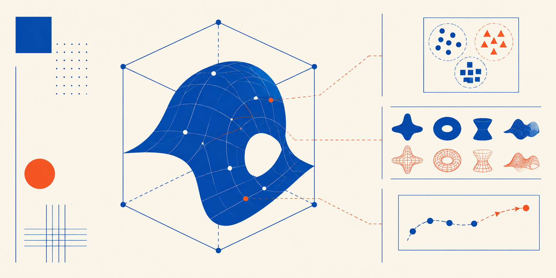
In this article, you will learn what latent spaces are and how they serve three distinct roles — descriptive, generative, and predictive — across a wide range of machine learning applications.
Topics we will cover include:
- How latent spaces compress high-dimensional data into structured numerical representations using techniques like Principal Component Analysis.
- How the generative role of latent spaces enables the creation of entirely new data points through interpolation.
- How the predictive role of latent spaces powers similarity-based applications such as recommender systems and RAG pipelines.
Introduction #
Think of a “secret”, multi-dimensional map in which machine learning models treasure the “essence” of complex, real-world data. That’s the primary purpose of latent spaces: compressed, numerical data representations containing the abstract features and hidden relationships of the original, raw data they come from — be it raw image pixels, audio, text, or simply high-dimensional, structured data like customer behavior history.
This article analyzes, illustrates, and categorizes the core functions and role of latent spaces in machine learning models. In particular, we distinguish between three roles: descriptive, generative, and predictive. Let’s unveil how latent spaces work under each of these hats through some concise, runnable code examples you can easily test in a Python notebook.
1. The Descriptive Role: Structuring and Representing Data #
Complex data normally needs to be summarized and structured in a more digestible form before feeding it to downstream machine learning models, extracting meaningful information into relevant features and discarding irrelevant or redundant ones. That’s the purpose of the descriptive role in latent spaces: a feature extractor compresses high-dimensional inputs into key traits, encoding them numerically. For example, in a dataset of raw, high-quality portrait images, disentangling factors like the subject’s pose or lighting keeps background noise aside while the core semantic information is preserved.
One particular technique that is widely used to compress high-dimensional data into a lower-dimensional space (a smaller number of features, in simpler terms) is Principal Component Analysis, or PCA for short. While PCA doesn’t extract tangible features like lighting or pose, it’s still a very popular technique to drastically compress the original data features (based on algebraic projections) while minimizing the loss of important information describing the original data — this important information underlying the original data is commonly known as variance in the context of PCA and dimensionality reduction techniques as a whole.
This example shows how to apply PCA to compress 3D data into a 2D latent space that maintains the original 3D data’s descriptive properties and relationships as much as possible:
from sklearn.decomposition import PCA
import numpy as np

raw_data = np.array([[1.1, 2.2, 3.3],
                     [1.0, 2.1, 3.1],
                     [8.1, 9.2, 9.9]])

pca = PCA(n_components=2)
latent_space_map = pca.fit_transform(raw_data)

print("Descriptive Latent Space (Compressed Data):\n", latent_space_map)

12345678910111213

from sklearn.decomposition import PCAimport numpy as np # Raw high-dimensional data: 3 items, 3 features per itemraw_data = np.array([[1.1, 2.2, 3.3],                      [1.0, 2.1, 3.1],                      [8.1, 9.2, 9.9]]) # Compressing into a 2D Latent Space mappca = PCA(n_components=2)latent_space_map = pca.fit_transform(raw_data) print("Descriptive Latent Space (Compressed Data):\n", latent_space_map)
Output:
Descriptive Latent Space (Compressed Data):
 [[-3.88962445e+00  4.39634517e-02]
 [-4.11856576e+00 -4.31334646e-02]
 [ 8.00819021e+00 -8.29987064e-04]]

1234

Descriptive Latent Space (Compressed Data): [[-3.88962445e+00  4.39634517e-02] [-4.11856576e+00 -4.31334646e-02] [ 8.00819021e+00 -8.29987064e-04]]
The example is extremely simple to illustrate the concept, but in practice, you might apply PCA to compress thousands of features into, say, a couple hundred at most.
2. The Generative Role: Creating New Data #
Obtaining latent space representations from data can also be leveraged as a canvas for creating completely new data instances. The generative role consists of creating new data points by randomly sampling feature values that “make sense” for such points, or by interpolating between existing ones. The key aspect to grasp here is: which values make sense for every feature — in other words, how do the values in each latent space feature distribute? Think of it, in its simplest form, as taking a mathematical stroll between two different existing points and blending their respective feature values in infinitely many ways to create whole new outputs: new points, such as images.
This is the core idea behind modern AI image generators, voice synthesizers, and so on. These systems rely on generative deep learning models like autoencoders, adversarial models, or even transformers. While these are remarkably complex and sophisticated models, their core ideas are based on interpolating points in a latent space, as shown in the code below:
point_a = latent_space_map[0]
point_b = latent_space_map[2]

generated_latent_point = 0.5 * point_a + 0.5 * point_b

generated_raw_data = pca.inverse_transform(generated_latent_point)

print("Newly Generated Data Point:\n", generated_raw_data)

1234567891011
Output:
Newly Generated Data Point:
 [4.6 5.7 6.6]

12

Newly Generated Data Point: [4.6 5.7 6.6]
Take this mathematical concept to the extreme, and you get something like an AI that can modify a person’s eye color in a provided image to make it darker or brighter, for instance.
3. The Predictive Role: Similarity and Forecasting #
How does the AI behind recommender engines guess what video you want to watch next? Or how does it efficiently and reliably identify your facial traits through the immigration gates on arrival at a destination airport after a long-haul flight? Latent spaces enter the scene again. The story is partly familiar: high-dimensional, complex data like user behavior history or high-resolution images are compressed into a latent representation for more efficient and effective management while retaining key characteristics. On top of that, the predictive role uses latent space coordinates to calculate similarities among data points, draw decision boundaries, and forecast outcomes like the most probable next video to watch or the closest-matching face to the one in front of the security camera.
In a video recommender system, for example, videos clustered near each other share key traits, making it easier to classify them, segregate them into categories, or fuel accurate, relevant recommendations.
This example code shows how to use cosine similarity to predict the most closely related data point to a new user input:
from sklearn.metrics.pairwise import cosine_similarity

new_item_latent = np.array([[0.0, 1.0]])

similarity_scores = cosine_similarity(new_item_latent, latent_space_map)

print("Predictive Similarity Scores:\n", similarity_scores)

12345678910

from sklearn.metrics.pairwise import cosine_similarity # A new, unknown item mapped into the latent spacenew_item_latent = np.array([[0.0, 1.0]]) # Measuring similarity between the new item and our existing latent mapsimilarity_scores = cosine_similarity(new_item_latent, latent_space_map) # Higher score equals closer geometric relationship in latent spaceprint("Predictive Similarity Scores:\n", similarity_scores)
Output:
Predictive Similarity Scores:
 [[ 0.01130203 -0.01047236 -0.00010364]]

12

Predictive Similarity Scores: [[ 0.01130203 -0.01047236 -0.00010364]]
This similarity-based and predictive principle is also leveraged in modern LLM-based applications like RAG systems, in which a user query is translated into a numerical latent representation called an embedding, and its similarity to existing document embeddings in a large database is calculated to retrieve the most semantically relevant texts to the original query.
Wrapping Up #
Whether you aim to describe the main characteristics of a dataset, generate novel art, or predict the next favorite video to watch, latent spaces are a valuable, foundational concept throughout the machine learning landscape. Mapping messy, real-world data into structured numerical representations is the master recipe for compressing, building, and connecting ideas across a wide variety of applications.