We recently released Quail, an execution engine for AI-SQL. One of the most common AI-SQL operations is classification: given a document and a list of labels, pick the label that fits best. E.g., a support team might want to sort every incoming message into “billing”, “refund request”, “shipping delay”, and so on.
Most systems classify a document the same way they answer any other question. They put the document and the labels into a prompt, let the LLM generate a response, and then parse the response into a label. The documentation of BigQuery’s AI.CLASSIFY and Snowflake’s AI_CLASSIFY describes a similar interface: each function adds a prompt to the input, sends it to an LLM, and returns the category that best fits. But letting the LLM generate freely is both wasteful and fragile — the LLM can spend many tokens on its response, and the response may not even contain a valid label!
Since Quail runs the LLM inside its own inference engine, it doesn’t have to let the LLM generate freely. Instead, Quail can restrict the LLM to the labels, and it turns out there are several ways to do so, each with a different cost. In this article, we discuss: For a given LLM, how should Quail execute AI.CLASSIFY?
We’ll go through:
- How
AI.CLASSIFYworks in Quail (Section 2 ). - Three ways that Quail can execute
AI.CLASSIFY: generating the label greedily, scoring all labels at once, and scoring one letter per label (Section 3 ). - How to estimate the cost of each way, building on our blog post on AI-powered filters , and how Quail picks the cheapest one (Section 4 ).
- An aside on decision models, which are LLMs fine-tuned to pick among answers (Section 5 ).
AI.CLASSIFY takes a document and a list of labels. It returns one of the labels.
Here is the query that we use throughout the post, with Qwen3-4B-fp8 as the LLM. It sorts support messages into 10 topics:
SELECT m.id,
       AI.CLASSIFY(
         m.body,
         ARRAY['billing', 'refund request', 'refund status',
               'shipping delay', 'shipping damage',
               'shipping address change', 'product defect',
               'two-factor authentication issue', 'praise', 'other']
       ) AS topic
FROM messages m;
The function has three arguments:
- input : the document to classify. Here, the input is the text of a support message.
- categories : 2 to 255 labels. Each label can have a short description of up to 25 words.
- options (not in the example query): an object with optional settings.
task_description: extra instructions for the LLM, up to 50 words.probabilities: whentrue, Quail also returns the columntopic_probabilities, with one probability for each label. The probabilities sum to 1.selectivity: an estimate of the fraction of rows that a condition on the label keeps, e.g.,WHERE topic = 'billing'. The optimizer uses the estimate to plan the query. The estimate does not change the labels.
Quail always returns one of the labels.
AI.CLASSIFY can also appear in a WHERE clause. E.g., the following query keeps only the messages about refunds:
SELECT m.id
FROM messages m
WHERE AI.CLASSIFY(m.body, ARRAY[...]) IN ('refund request', 'refund status');
A condition on the label uses = or IN. When the same classification appears in SELECT and in WHERE, Quail runs the classification only once.
In database terms, AI.CLASSIFY is a logical operator. Quail supports three physical implementations of the operator, and the optimizer selects one implementation for each query.
All three implementations send the LLM one prompt for each document. The prompt starts with DOCUMENT: and the document. Then it has a question with the list of labels. After the prompt comes the token ANSWER:, where the LLM scores the first token of the answer. The prompts of the three implementations differ slightly in the question and the label list, as shown in Figure 1.
The implementations also select the label in different ways. trie_decode generates the label token by token, trie_tree scores every label in one request, and letters scores one letter for each label.
3.1 trie_decode: Greedily Generate the Label #
trie_decode is the implementation that is closest to what prior systems do. It generates the label one token at a time, as an LLM generates text.<sup>1</sup> At each decode step, the LLM picks the most likely token that continues a label.
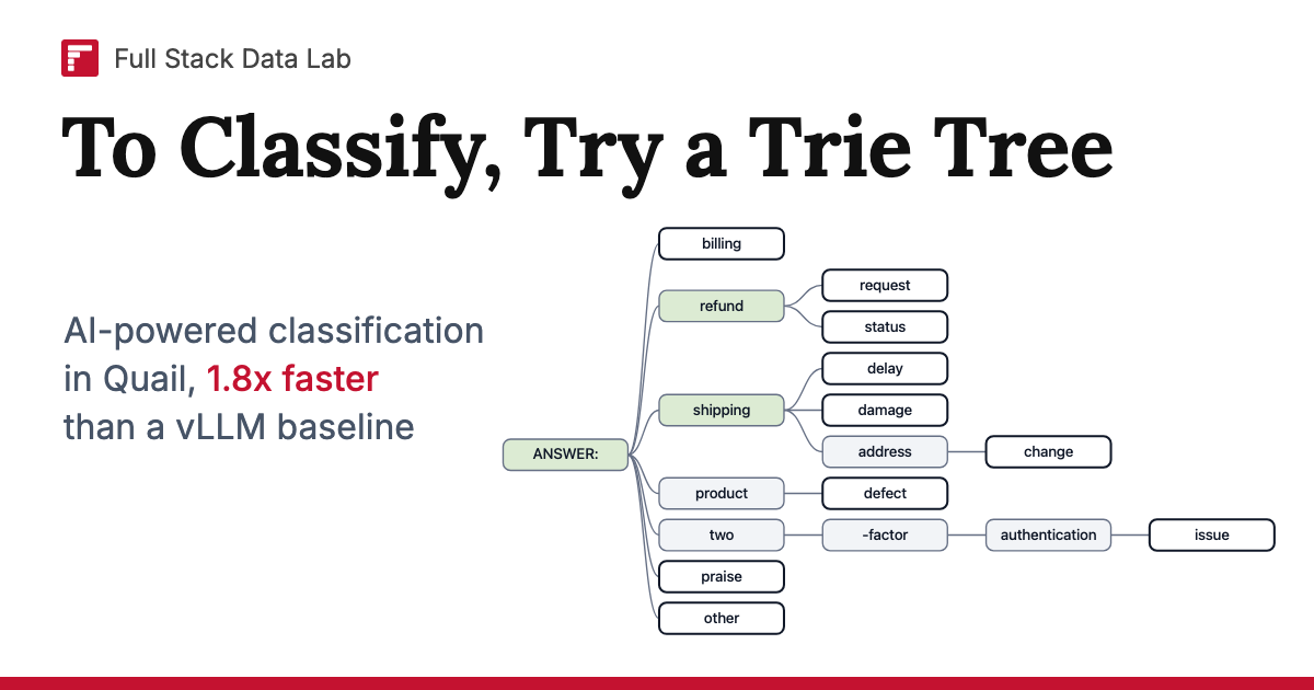
At a high level, we can assemble the set of labels into a trie (Figure 2). A trie, also called a prefix tree, stores each label as a path of tokens from the root. Labels that start with the same tokens share the start of their paths, e.g., both refund labels pass through refund. The root of the trie is the ANSWER: token. For the rest of the article, we write labels in quotes and tokens in code, e.g., the label “refund request” has the tokens refund and request.
The simple way to generate a label is one token per decode step. At each decode step, the LLM reads the tokens so far and picks the most likely child of the current node in the trie. E.g., to generate “shipping address change”, the LLM could take 3 decode steps. It would pick shipping at ANSWER:, then address, and then change.
Now, you might realize — if the answer really was “shipping address change”, by the time we are at the second decode step (address), we actually need not decode the change token, because there is no other valid token!
More generally, the LLM only needs to make a choice where the labels branch apart in the trie, i.e., at a node with more than one child. In our running example, there are only 3 such nodes: ANSWER: (which first word?), refund (request or status?), and shipping (delay, damage, or address?). Everywhere else, the next token is already determined. So Quail only runs the LLM at the 3 branching nodes, and it stops as soon as there’s just one label left. For instance, if the LLM picks product at ANSWER:, the answer must be “product defect”, so one step and we’re done!
What does this look like when we classify many documents at once? Figure 3 shows the decode steps for a batch of 10 documents. Quail computes each step for all documents in the batch together, in one forward pass. Step 0 happens in the same request as the prompt: the LLM reads the document and picks the first token at ANSWER:. Then, each later decode step sends one more request, but only for the documents whose labels aren’t decided yet. In our running example, only the 5 documents that picked refund or shipping need a step 1, and the other 5 documents are already done.
So trie_decode is pretty cheap: if every label is equally likely, a document in our running example needs just 1.5 requests on average. But there is a catch — since it is greedy, trie_decode only looks at the tokens on its own path. It never scores the other labels, so it can’t return label probabilities. So, if the user asks for probabilities, Quail must use one of the other methods.2
3.2 trie_tree: Score All Labels at Once #
What if the user wants probabilities? A simple approach would score every label with its full probability under the LLM. The probability of a label is the product of the probabilities of its tokens. If label $m$ has the tokens $x_1, \dots, x_t$, then
$$ P(m) = \prod_{k=1}^{t} P(x_k \mid \text{prompt}, x_1, \dots, x_{k-1}). $$ E.g., for “refund request”,
$$
P(\text{refund request}) = P(\texttt{refund} \mid \text{prompt}) \times P(\texttt{request} \mid \text{prompt}, \texttt{refund}).
$$
However, the simple approach would unfairly penalize longer labels. Each extra token multiplies the score by a number below 1, even after the label is already decided. E.g., the score of “shipping address change” would include the probability of change, although change is the only token that can follow address.
So in trie_tree, we only score each label until we know which label it is. More precisely, we score the tokens up to the end of the word where the label branches away from all the other labels. Let $d_m$ be the position of the last token of the word in label $m$. Then
To illustrate, here are the scores of three labels in the running example. To keep the table short, we leave “prompt” out of each probability:
| Label | Score |
|---|---|
| shipping address change | $P(\texttt{shipping}) \times P(\texttt{address} \mid \texttt{shipping})$ |
| product defect | $P(\texttt{product})$ |
| two-factor authentication issue | $P(\texttt{two}) \times P(\texttt{-factor} \mid \texttt{two})$ |
“shipping address change” branches away from the other labels at “address”, because “delay” and “damage” also follow shipping. “product defect” branches away at “product”, because no other label starts with product. “two-factor authentication issue” branches away at “two-factor”, which is one word with two tokens, so we score both tokens.
Next, we have to convert the scores into probabilities. The 10 scores won’t add up to 1, because at every token, the LLM spreads its probability over all 151,936 tokens in its vocabulary, including tokens that aren’t part of any label, like The. So Quail divides each score by the sum of all 10 scores:
Here, $\hat{P}(m)$ is the probability that Quail returns for label $m$.
Finally, we have to handle the scenario where one label is the start of another label. The running example has no such labels. Hypothetically, imagine that we had both “refund” and “refund request” as labels. After refund, the LLM can stop, which means the answer is “refund”, or it can continue with request. So the score of “refund” is the probability of refund times the probability of not continuing with request:
Otherwise, the probability of refund would count toward both labels.
Now, back to the running example. Like in trie_decode, we could run the LLM at every trie node that has children, which is 8 nodes. However, similarly to trie_decode, running the LLM at every such node is not as efficient as it could be. You might expect trie_tree to need only the 3 branching nodes, like trie_decode. But it needs one more token, two! Otherwise, the score of “two-factor authentication issue” would also include the probability of other text that starts with two, such as “two days ago”. So we multiply by the probability of -factor after two. So trie_tree runs the LLM at 4 nodes (ANSWER:, refund, shipping, and two), all in the same request as the prompt.
Custom attention kernel. Lastly, consider how to execute the algorithm above on the GPU. A simple way is to send 4 requests to the LLM, each containing the same prefix (prompt and label descriptions) followed by a different trie node to compute the probability of. Sure, the KV of the prefix may be shared across the 4 requests, but each request would still read the KV of the whole prefix from GPU memory. Instead, Quail sends all 4 nodes in one request to the LLM, using a custom tree attention kernel.<sup>3</sup> Each node attends only to the prompt and to the nodes on its own path, as shown in Figure 4.
Overall, trie_tree always processes at least as many tokens as trie_decode, because it runs the LLM at the branching nodes of every label. However, trie_tree needs only one request per document.
3.3 letters: Score One Token per Label #
There’s an even simpler way to get probabilities: turn every label into a single token.4letters puts a letter before each label in the prompt (“A: billing”, “B: refund request”, and so on) and asks the LLM for the letter instead of the label, as shown on the right side of Figure 1. Now Quail needs just one step. At ANSWER:, it reads the probabilities of the 10 letters, rescales them so they sum to 1, and picks the label whose letter has the highest probability. So there’s no trie and no extra request.
The downside is a longer prompt, because every label line now has a letter. Accuracy can also change, because the LLM has to answer with a letter instead of the label itself.5
3.4 Keeping the Document KV for Later Operators #
So far, we’ve looked at one AI.CLASSIFY call on its own. But real queries often run several AI operators over the same documents. E.g., a query might classify the topic of each message, keep only the refund messages, and then classify how urgent they are. Every operator reads the same message, so it would be wasteful to process the message from scratch each time.
Instead, Quail stores the KV of each document in its KV cache, so the next operator only has to process its own question, even when the operators have different semantics (e.g., a filter, a classification, and a join). Of course, GPU memory is limited, so Quail can’t keep the KV of every document around forever. When memory fills up, Quail evicts the KV that it expects to save the least work per page.6
So which method should Quail use? In short, when trie_decode can run, it is usually the fastest, assuming that Quail packs every forward pass full of tokens. But trie_decode is not always the fastest, and the user may also ask for probabilities, which trie_decode can’t give. So here, we’ll walk through the cost of each method, to see where the differences come from.
Like all cost models in Quail, our cost models for classification are based on speed-of-light (SoL) estimates, i.e., the lowest possible time of the work on the GPU. Our blog post on AI-powered filters explains SoL estimates in detail, and we reuse its notation: $N$ is the number of documents, $\ell_i$ is the number of tokens in document $i$, and $K$ is the number of forward passes.
4.1 Workload and Notation #
Table 1. Symbols in the classification cost model. #
| Symbol | Meaning |
|---|---|
| $N$, $\ell_i$, $L_1$ | Number of documents, tokens in document $i$, and total document tokens |
| $q_{\text{pre}}$, $q_{\text{tail}}$ | Tokens in the preamble and in the instruction (question and label list) |
| $a$ | Expected answer positions per document |
| $r_i$, $n_{\text{tok}}$ | Tokens in the request for document $i$, and in all requests |
| $C$, $K$ | Token budget of one forward pass, and number of forward passes |
| $M$, $c_m$, $b$ | Number of labels, branching nodes on the path of label $m$ up to the one that decides it, and expected number of requests of trie_decode per document |
| $B_{\text{kv}}$, $R$ | KV bytes per token, and saved KV tokens that the answer positions read |
| $d_{\text{model}}$, $\text{vocab}$ | Width of the hidden state, and number of tokens in the vocabulary |
| $V_{\text{out}}$ | Rows of the output head that Quail computes at each answer position |
| $T_{\text{head}}$, $T_{\text{classify}}$ | Estimated latency of the output head, and of one classification |
Let’s start by setting up some notation. Recall from Section 3 that Quail sends the LLM one request per document. The request contains the preamble (the text DOCUMENT:), the document, the instruction (the question and the list of labels), and then the answer positions. An answer position is a token after the instruction where Quail reads the scores that the LLM gives to the next token, like the ANSWER: token.
Let $q_{\text{pre}}$ and $q_{\text{tail}}$ be the number of tokens in the preamble and the instruction. Let $a$ be the expected number of answer positions per document, and let $s$ be the expected number of answer positions where Quail reads scores. Then the request length, the total number of tokens, and the number of forward passes are
$$ \begin{aligned} r_i &= q_{\text{pre}} + \ell_i + q_{\text{tail}} + a, \ n_{\text{tok}} &= L_1 + N(q_{\text{pre}} + q_{\text{tail}} + a), \ K &= \left\lceil \frac{n_{\text{tok}}}{C} \right\rceil. \end{aligned} $$ Here, $L_1 = \sum_i \ell_i$ is the total number of document tokens, and $C$ is the maximum number of tokens in one forward pass.
The three methods only differ in $q_{\text{tail}}$ and $a$. Table 2 gives the values for our running example.
| Method | $q_{\text{tail}}$ | $a$ |
|---|---|---|
trie_decode |
66 | 1.5 |
trie_tree |
66 | 4 |
letters |
89 | 1 |
For projections, attention, and the MLP, we can reuse the formulas from our blog post on AI-powered filters, plugging in the new $n_{\text{tok}}$ and $r_i$. However, classification differs from filters in two ways: (1) each method has a different number of KV reads, i.e., loads a different number of cached KV tokens, and (2) classification needs the whole output head, i.e., scores for the whole vocabulary, not just TRUE and FALSE.
KV reads. Each answer position attends to the prompt, so the GPU has to load the KV of the prompt from HBM. letters and trie_tree load it once per document, since all of their answer positions are in one request. trie_decode loads it once per extra decode step. Step 0 shares the request of the prompt, but every later decode step is a new request. So if $b$ is the expected number of requests of trie_decode per document (including step 0), the number of KV tokens loaded is
Plugging $R$ into the formula from our blog post on AI-powered filters, attention moves $B_{\text{attn}} = B_{\text{kv}}(W + R)$ bytes. Here, $B_{\text{kv}}$ is the number of KV bytes for one token across all layers, and $W$ is the number of tokens whose new KV attention writes.
Output head. After the last layer, each answer position has a hidden state, which is a vector of $d_{\text{model}}$ values. The LLM turns the hidden state into a score for every token in its vocabulary, using one more matrix multiplication. We call the matrix the output head.<sup>7</sup> The output head has one row for each vocabulary token, so the score of a token is just the dot product of the hidden state with the row of the token.
Let $V_{\text{out}}$ be the number of rows that Quail computes at each answer position. If every label is a single token (like the letters in letters), Quail only computes the rows of the label tokens. Otherwise, Quail computes all $\text{vocab}$ rows, which it needs to turn the scores into probabilities. Since the output head is in BF16,
Here, $F_{\text{head}}$ counts two FLOPs per value of each computed row at each answer position, and $B_{\text{head}}$ counts two bytes per value of each computed row in each forward pass. $\Pi_{bf16}$ and $\beta$ are the peak BF16 throughput and the HBM bandwidth of the GPU. For Qwen3-4B, $d_{\text{model}} = 2{,}560$ and $\text{vocab} = 151{,}936$.
The SoL estimate of one classification is
$$ T_{\text{classify}} = T_{\text{proj}} + T_{\text{attn}} + T_{\text{mlp}} + T_{\text{head}}. $$ Here, $T_{\text{proj}}$, $T_{\text{attn}}$, and $T_{\text{mlp}}$ are the estimated latencies of the projections, attention, and the MLP.
4.2 Cost of trie_tree and letters #
trie_tree and letters each put all of their answer positions in the same request as the prompt, so they only differ in how many tokens they add to each document.
For trie_tree, each answer position is one more token that goes through the whole LLM, which costs about 7.2 billion FLOPs in the projections and the MLP, just like a document token. Since some labels have more than one token, Quail also computes the full output head at each answer position, which adds about 0.78 billion FLOPs. In our running example, trie_tree has 4 answer positions, so it adds about 32 billion FLOPs per document ($a = 4$ and $V_{\text{out}} = \text{vocab}$).
For letters, the extra tokens are in the prompt instead. The letters add $2M + 3$ tokens to the instruction, where $M$ is the number of labels. Each label line gains 2 tokens for its letter, and the question gains 3 tokens for the words “the letter of”. In our running example, the letters add 23 tokens, which cost about 166 billion FLOPs per document. The output head is cheap, because Quail only computes the 10 rows of the letters ($a = 1$ and $V_{\text{out}} = M$). So in our running example, the extra work of letters is about 5 times the extra work of trie_tree. However, both are small next to the document itself, which costs about 7 trillion FLOPs for a 1,000-token document.
4.3 Cost of trie_decode #
Unlike the other two methods, the cost of trie_decode depends on which label the LLM picks, because some labels need more decode steps than others. Quail doesn’t know the labels before it runs the query, so the cost model assumes that every label is equally likely.8
Each branching node on the path of a label costs one request. So if $c_m$ is the number of branching nodes on the path of label $m$, up to and including the one that decides the label, the expected number of requests per document is
$$
b = \mathbb{E}[\text{requests per document}] = \frac{1}{M} \sum_{m=1}^{M} c_m.
$$
In our running example, 5 labels are decided right at ANSWER:, and the other 5 need one more branching node ( refund or shipping), as shown in Figure 3. So
In our running example, each decode step adds a single token after the prompt: ANSWER: in step 0, and refund or shipping in step 1. So trie_decode runs the LLM on 1.5 tokens per document on average, beyond the prompt. Like for trie_tree, each token costs about 8 billion FLOPs (7.2 billion in the projections and the MLP, plus 0.78 billion for the full output head). So trie_decode adds only about 12 billion FLOPs per document, compared with about 32 billion for trie_tree.
Note that the estimate assumes optimal packing, i.e., that Quail packs many documents together so that each forward pass saturates the GPU.<sup>9</sup> With only a few documents, a later decode step can run in a nearly empty forward pass, and trie_decode costs more than the estimate.
4.4 Picking a Method #
Putting it all together, the optimizer computes $T_{\text{classify}}$ for every method that can run, and it picks the method with the lowest estimate.
In our running example, trie_decode wins, because it runs the LLM on the fewest extra tokens per document: 1.5, compared with 4 for trie_tree and 24 for letters. letters only wins when there are a few labels that share a long start, e.g., 2 labels that differ only in their last word, since both trie methods have to run the LLM on every shared token. And trie_tree mostly wins when the query asks for probabilities, since trie_decode can’t run then.
Note that the differences are small, between 2% and 11% for 1,000 documents of 100 tokens, because all three methods have to prefill the preamble, the document, and the instruction, and the prefill is most of $T_{\text{classify}}$.
4.5 Experiments on QUAIL-B #
To see how all of this plays out end to end, we added 12 classification queries to QUAIL-B, our benchmark for AI-SQL. The queries span five datasets (movie reviews, adverse drug event reports, fact-checking claims, legal citations, and agent traces), with 4 to 27 labels for each AI.CLASSIFY operator. Some queries have only one operator (AI.CLASSIFY); other queries also have filters, joins, or multiple different AI.CLASSIFY operators.
We ran each query with Qwen3-4B-fp8 on one H100, at scale factor 0.5, on both Quail and a vLLM baseline (v0.26.0, with prefix caching). In the vLLM baseline, the LLM generates the label, and then we parse it. Figure 6 shows the results.
Quail is faster on all 12 queries: 2.1x faster in total, and 1.8x faster per query (geometric mean). The biggest wins come from queries that read the same documents more than once. E.g., AGENT-5 has three different AI.CLASSIFY operators on the same agent traces. vLLM’s prefix cache evicts the least recently used KV, so by the time the next operator reads a trace, its KV is usually gone and vLLM has to recompute it. On AGENT-5, 64% of the tokens that vLLM computes are recomputations. Quail instead keeps the KV of the trace around for the later operators (Section 3.4). Quail also runs within 1.8x to 2.8x of its SoL estimate on every query.
Last month, TypeSafe AI released Jev, a decision model. Instead of generating text, Jev answers a typed question (e.g., yes or no, or pick one of a few labels) and returns a probability for each answer. Jev took the community by storm, and open follow-ups came out within weeks: Kev from Jared Palmer, Clef from Cloudflare, and the Decision models from the vLLM Semantic Router team. Databricks even runs open decision models in SQL. Quail supports one of the open models, Decision 2.0 Kai 0.6B, as an alternative to the three methods above.
Decision 2.0 Kai is a fine-tuned version of Qwen3-0.6B. It never generates text; it just returns a probability for each answer, in one forward pass.
Let’s briefly walk through how it works, as shown in Figure 5. Instead of listing the labels in the instruction, Quail writes each label into its own option block after the document. The LLM runs on the whole prompt as usual, and each token comes out of the last layer as a hidden state. Then, an extra decision head reads the hidden state $h_m$ of the last token of each option block $m$, and the hidden state $q$ of the last token of the prompt.
The decision head first rescales $h_m$ and $q$ so that their values are on a similar scale, giving $\bar{h}_m$ and $\bar{q}$. Then, it computes a score $s_m$ for each label $m$, and a softmax turns the scores into probabilities:
$$ \begin{aligned} s_m &= \frac{(W_h \bar{h}m) \cdot (W_q \bar{q})}{\sqrt{d}} + w \cdot \operatorname{GELU}!\left(U_h \bar{h}m + U_q \bar{q} + b\right), \ P(m) &= \frac{e^{s_m}}{\sum{j=1}^{M} e^{s_j}}. \end{aligned} $$ The first term is a dot product, like an attention score, and the second is a tiny neural network. $W_h$, $W_q$, $U_h$, $U_q$, $w$, and $b$ are weights learned during fine-tuning. The $W$s and $U$s are $d \times d{\text{model}}$ matrices that shrink the hidden states down to $d$ values, and $w$ and $b$ are vectors of $d$ values that turn the GELU output into a scalar.<sup>10</sup> For Decision 2.0 Kai, the whole decision head has about 1 million weights, compared with about 600 million in the LLM, so it costs almost nothing.
Like trie_tree, Decision 2.0 Kai gives probabilities in one request. But trie_tree has to score every token in the vocabulary at each answer position, while Decision 2.0 Kai only scores the $M$ labels.
One might notice that the option blocks add a lot of tokens: about 16 tokens per label, or about 190 tokens per document in our running example, compared with 24 for letters. But the extra tokens (more specifically, the trained decision head) buy a lot of accuracy. We ran Decision 2.0 Kai and the base Qwen3-0.6B on the 12 classification queries in QUAIL-B, on one H100. Decision 2.0 Kai agrees with the reference labels on 63.1% of documents on average, compared with just 39.0% for Qwen3-0.6B! We are really excited about these decision models and believe we can fine-tune our own decision models for AI-SQL tasks (potentially even-smaller models).
In this article, we walked through the many ways to execute AI.CLASSIFY. Since Quail runs the LLM inside its own inference engine, it can restrict the LLM to the labels: it can greedily generate the label (trie_decode), score all labels at once ( trie_tree), or score one letter per label ( letters), and it picks whichever is cheapest for the given LLM and labels. Most of the time, the answer is a trie: trie_decode by default, and trie_tree when the query asks for probabilities.
Next, we’re working on supporting bigger decision models (built on hybrid architectures) and new operators like AI.EXTRACT. Stay tuned for more exciting stuff! In the meantime, try out Quail, and if you like what we’re building, give it a star on GitHub!
We thank Modal for sponsoring the compute used in this research.
1. Prior open-source LLM-powered data processing systems from academia, such as DocETL, LOTUS, and Palimpzest, also have the LLM generate the answer token by token.
2. Moreover, we also have to use one of the other methods if one label is an exact prefix of another label. E.g., suppose the labels are “refund” and “refund request”. After refund, the label could already be complete, or it could continue with request. trie_decode picks the next token, but we do not define a token for stopping. So trie_decode can never pick the label “refund”.
3. Our blog post introducing Quail describes the tree attention kernels for AI joins. In a join, many partner documents share one anchor document. In trie_tree, many trie nodes share one prompt.
4. The structured mode of DiffusionGemma in vLLM uses the same idea. It accepts only one-token choices, and it maps longer options to letters, e.g., “moderation_spam” to “A” (vLLM PR #57250).
5. We don’t know which method is the most accurate in general. On two of our QUAIL-B queries, trie_tree and trie_decode agree with the reference labels about equally often (72.1% vs. 72.0% on BIO-5, and within 0.2 points on AGENT-5). For the purposes of the post, we assume that all three methods are about equally accurate, and we expect strong open LLMs to make all three good enough for most queries.
6. Quail estimates the savings of a page as the probability that a later operator reads the document, times the time to process the document again, divided by the number of pages of the document. See the Quail documentation on KV retention.
7. It’s fine for our blog post on AI-powered filters to leave the cost of the output head out of its cost model, because a filter only needs the rows for TRUE and FALSE, at most 8 rows when we count spellings like True, instead of all 151,936 rows. The 8 rows cost about 41,000 FLOPs per document, while each document token takes about 7.2 billion FLOPs in the projections and the MLP.
8. The real labels are usually not equally likely, so the estimate of $b$ can be too high or too low. E.g., suppose most documents get a label that is decided at the ANSWER: token. Then trie_decode sends fewer requests than the estimate, so the SoL estimate of trie_decode is too high.
9. This is pretty different from online serving engines like vLLM. vLLM cares about the latency of each request, so it runs decode steps as soon as it can, even in mostly empty forward passes. Quail doesn’t care about the latency of each individual document, just the latency of the whole query, so it can always fill the forward pass.
10. We found the decision head described in decision_model.py, the code that ships with the model on Hugging Face.
@misc{shankar2026aiclassify,
  title = {To Classify, Try a Trie Tree},
  author = {Shankar, Shreya and Frye, Charles},
  year = {2026},
  month = oct,
  url = {https://fsdatalab.github.io/blog/ai-classification/}
}