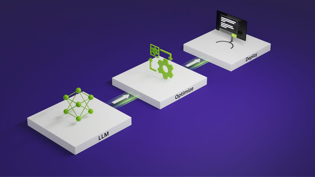
Last week I spent some time diving more into LLM inference. This is a field I personally find interesting, especially because of the optimizations and engineering behind it. It is a tricky optimization problem where the goal is to make LLM inference possible while controlling hardware costs and keeping high quality.
This is post will also find relevant those who want to run open source LLMs on their own infrastructure. There might be multiple reasons to do that, such as cost control to avoid unpredictable per-token pricing, data privacy to keep sensitive data-in-house, lower latency by serving models closer to where the data lives, and greater flexibility to fine-tune or customize models without depending on a third-party provider's roadmap or rate limits among others.
However, the knowledge required to run those workloads is vast and requires understanding the underlying mode of operation of Large Language Models (LLMs), especially the popular transformer architecture and the SOTA (State of the Art) advances in this area. Let’s dive in.
The planning Phase #
First, you have to choose a model for your use case. This is a planning process where you must involve AI engineers, business owners, infra engineers, and DevOps engineers with LLMOps experience. It is very important to know the nuances of choosing different models depending on the business use case.
For the sake of keeping this article short, let’s say you have decided to give it a try with Llama3.1 8B. Before taking any further steps, let’s check what it means by choosing this model.
- It is a multilingual LLM . It means this model was trained on diverse, multilingual datasets. Hence it has inherit the capacity to do translation.The multilingual part is probably not necessary for your use-case.
- This is a text in/text out model. It does not handle images, audios, videos or any other sort of inputs. Only text as input and produce only text as output.
- It uses a transformer architecture . This is very important to know in advance because there are inference servers that support only transformers.
- The model uses Grouped-Query Attention (GQA) for enabling fast inference.
- Context length: 128k . This is also very important though 128k of context length is quite long. Ok it depends. For example, if you are planning to use the LLM as a code agent the context length could exponentially grow. Since in the model card say that it support 2 output modalities: Multilingual text and code. We expect the context length to be big enough for using for coding agents.
- Supported languages: English, German, French, Italian, Portuguese, Hindi, Spanish, and Thai.
I was able to gather all of the above information from the model card. Now we need to have an idea of what it will take in terms of resources to run this model in production.
The Resource Estimation Phase #
One of the first questions you should have: How much memory will it take to store a model with 8B (billion) parameters in GPU memory (VRAM) using FP16 (half precision)?.
The formula to calculate the memory usage for the models weights (parameters) is the following:
It means that for a model with 8 billion of parameters at half precision (FP16) where each parameter occupies 2 bytes we have:
It means that to only store the model’s parameters we required at least 16GB of GCPU VRAM.
In order to have an idea how the VRAM is a bottleneck, we can see in the image below the GPU memory usage distribution when upgrading to a model with 13B of parameters.
We can immediately notice that using same hardware and upgrading our model we are reserving less memory space for KV cache which has an impact in model latency (negative), throughput (negative) and accuracy (probably positive due the increase of numbers of parameters). We will always need to make tradeoffs as shown in the figure below.
For each generated token, caches must stores a key and value vector per transformer layer and head. It is very important that you calculate and have an estimation of the potential KV usage.
One way to get this information without the model is checking the config.json in Hugging Face.
We will see that the variables names are slightly different but here are the naming conventions:
n_layers -> num_hidden_layers
n_heads -> num_attention_heads
d_model -> hidden_size
d_head = hidden_size / num_attention_heads
Doing the math, we can come with the result that for the Llama3.1 8B model in FP16 (2 bytes per element), we will need approximately 0,52MB per-token KV cache. For the full 131’072 (128k) context window, the KV cache size is about 68,7 GiB.
That is for Batch size equal to 1. When we increase the batch size, the total memory footprint scales linearly with each additional sequence.
Now we understand that the KV cache prevents us from generating very long sequences and from processing large batches. This is one of the main reasons we need to apply optimizations techniques like quantization (more on this later), KV cache offload, continuous batching and others we will see later.
As you might noticed, if we want to run full context of 128K for the 8B parameter Llama model we are using on this article and using the same hardware (NVIDIA A100 - 40 GB). We cannot run even 1 inference query. We will run in OOM. The only option is upgrade hardware, apply quantization or use a smaller model.
Optimizations #
In this section, I present a brief overview of the optimizations most commonly used in LLM inference. Most are already implemented in inference frameworks such as SGLang, vLLM and llm-d.
1-Paged Attention
First published in the now widely cited paper Efficient Memory Management for Large Language Model Serving with PagedAttention.
This is a technique to manage efficiently the KV cache memory of the GPU. It is inspired by the algorithm utilized in classical virtual memory and paging techniques in operating systems.
In earlier systems, KV cache allocation per request or batch reserved memory that went unused. Each allocation reserved space matching the context length limit for the duration of generation, which constrained batch size. PagedAttention improves the memory management, cutting waste to under 4% and increasing throughput by 2-3x.
2-Prefix Caching
This is a technique utilized to avoid redundant prompt computations. The approach is to cache the kv-blocks of processed requests, and reuse these blocks when a new request comes in with the same prefix as previous requests.
As shown in the image below we can see two scenarios when prefix caching is utilized. The first one is when different users utilized the same system prompt (for instance in RAG), this prompt is computed only the first time and then subsequently loaded from cache.
The second example is when a single user is having a multi-turn conversation with the LLM. The session length or context from previous rounds are cached and then subsequently loaded from cache to avoid to re-compute it again.
We can see in figure below how by using prefix-caching we can increase the throughput during inference.
3-Parallelism
There are multiple forms of parallelism within inference systems. This technique allow FLOP operations at different layers to be executed in parallel.
I am not going to go deeper into each on these forms but I will briefly mention them on this article.
Data parallelism: Groups multiple independent requests into batches.
Tensor Parallelism: This is a technique that split layer-wise the weights of transformer model and computations are assigned to independent GPU cores.
Pipeline Parallelism: Mostly used when using big LLMs with multiple GPUs nodes. Basically is a technique to partition the model layer-wise, assigning different layers to separate GPUs for computing.
3D Parallelism: Combined them all
There is also Expert Parallelism for Mixture-of-Experts (MoE) architecture but I am not going to talk about this one on this article.
From vLLM documentation they recommend when using vLLM the following approaches:
- Single GPU (no distributed inference): if the model fits on a single GPU, distributed inference is probably unnecessary. Run inference on that GPU.
- Single-node multi-GPU using tensor parallel inference: if the model is too large for a single GPU but fits on a single node with multiple GPUs, usetensor parallelism . For example, set tensor_parallel_size=4 when using a node with 4 GPUs.
- Multi-node multi-GPU using tensor parallel and pipeline parallel inference: if the model is too large for a single node, combinetensor parallelism withpipeline parallelism . Set tensor_parallel_size to the number of GPUs per node and pipeline_parallel_size to the number of nodes. For example, set tensor_parallel_size=8 and pipeline_parallel_size=2 when using 2 nodes with 8 GPUs per node.
4-Quantization
LLM model’s parameters are continuously growing. As shown before, it is required to stores all parameters in memory (GPU VRAM). This means the total model size sets the minimum memory requirement.
Quantization is a method to make models smaller to overcome this issue. Parameters are usually stored in floating-point numbers and inference involves a huge amounts of floating-point operations (FLOPS). There are different floating-point precisions such as FP32, FP16, BF16, INT8, INT4. By lowering the precision we massively reduce the memory usage but at the potential cost of reducing accuracy.
LLM compression improves both throughput and latency and done correctly, it does not significantly degrade the performance of the model.
5-Speculative Decoding
This is a technique to speed up inference. Due the fact that autoregressive generation will generate a single token for every full forward pass. This a sequential process resulting the GPU compute power to stay idle most of the time.
Speculative decoding is technique that combine a target model and a draft model (a more smaller one) in a mechanism where the draft model proposes multiple token for the next generation and the target model verifies those proposals (all of them) in a single forward pass.
Compared with standard autoregressive decoding, which produces on token per pass, this technique reduce the latency during inference and boosting the throughput without any impact on accuracy.
6-Cache Aware Routing
Often the LLM you need to deploy does not fit in a single GPU or even if it does you need multiple GPUs to increase the throughput of the system to be able to serve more users.
In a distributed system when an user send multiple requests during the same session usually you cache them in one server to reduce computing across the whole system.
In distribute inference for LLMs we do something similar. When user is interacting with the LLM asking questions, refining answers, perhaps the LLM is calling tools or sub-agents everything during the same session or context, you don’t want to recompute and cache the context every time and in all machines. This will be a waste of resources.
A technique to solve this is called KV cache aware routing. This mechanism makes intelligent routing decisions based on KV cache awareness.
The way it works is for example the user send a request to the router like this:
curl http://localhost:30080/v1/completions \
  -H "Content-Type: application/json" \
  -d '{
    "model": "meta-llama/Llama-3.2-1B-Instruct",
    "prompt": "What is the capital of France?",
    "max_tokens": 100
  }'
Then, send another request with the same prompt prefix:
curl http://localhost:30080/v1/completions \
  -H "Content-Type: application/json" \
  -d '{
    "model": "meta-llama/Llama-3.2-1B-Instruct",
    "prompt": "What is the capital of France? And what is its population?",
    "max_tokens": 100
  }'
You should observe that the second request is routed to the same instance as the first request. This is because the KV cache aware router detects that the second request shares a prefix with the first request and routes it to the same instance to maximize KV cache utilization.
Conclusions #
As you have seen it is not trivial to run LLMs in your own hardware. There are a lot of tweaks to make and decisions to take depending on your use-case. Also take this article as a basic reference as I am omitting more advanced techniques and I am not going tin depth on the ones mentioned in the article. Thanks for reading!
Sources