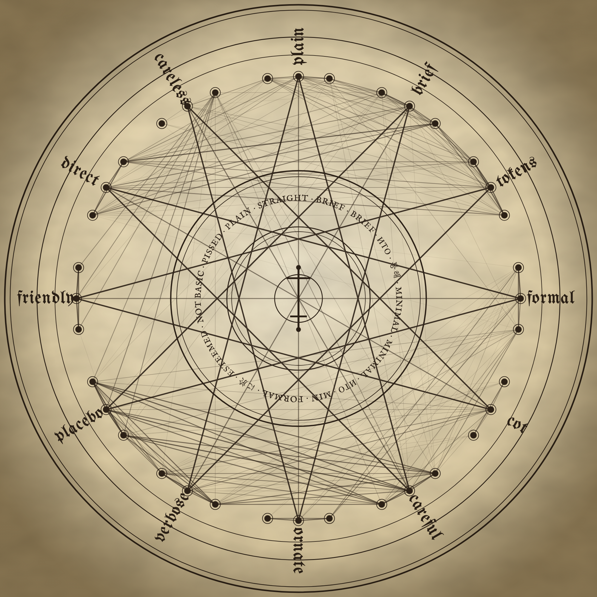
"Please Remove All Mannered Prose" and Other LLM Incantations

wpnews.pro

The Key of Solomon details incantations, prayers, and invocations that when said exactly right allow an adept to harness supernatural powers, including non-human intelligences. Messing up an incantation even slightly can result in disaster.

While using LLMs, I constantly add little modifiers to my main prompts to shift the model’s outputs to our preferred style. “Please be concise”, “avoid em dashes and semicolons”, “restrict inline comments to 8 words or less” and so on. These “style prompts” work pretty well, but I have found them unpredictable. Also, sometimes two “style prompts” that seem to mean the same thing to a human reader will change a model’s outputs in different ways. Anthropic recently posted some docs recommending adding Please remove all mannered prose to avoid the LLM “slop” tone that people have learned to tune out. It seems to work pretty well, but the strangeness (and Claudeness) of that phrase struck my curiosity and made me wonder about the other style prompts that I use while working with LLMs. It seems to me that to use LLMs better we need a more rigorous treatment of this subject.

How specific is a style prompt’s effect to its wording? Do style prompts similar to Please remove all mannered prose change llm outputs in similar ways?
How consistent is the effect of a style prompt across a set of different types of tasks?
How do Please remove all mannered prose outputs relate to outputs from an “opposite” style prompt such as Please use mannered prose? Can we characterize other “style prompt duals” in the same way?
Do these style prompts have the effects we intend?

To work effectively with LLMs, we need to understand how our inputs and context shift model outputs. Engineers can build single-purpose eval sets for heavily reused tasks, but at least in my world almost all prompts are too specific, urgent, or context-dependent to stop and build an eval set. Shipping models with more thorough quantitative documentation of how prompt modifiers and added context affect generated outputs could make them better “daily drivers” in these typical use cases.

Background #

If you are interested in this stuff, I recommend reading Stolfo et al., Improving Instruction-Following through Activation Steering (ICLR 2025). I will use a modified framework from that paper for this investigation. We will investigate these questions with three methodological tools: residual geometry a la Solfo et al. and Zou eta l., the logit lens a la nostalgebraist, and output stylometry using standard readability metrics (Flesch 1949, Guiraud’s 1954 book).

Approach #

To do this kind of interpretability work, we need to inspect a model’s intermediate state while it is responding. That means it needs to be open-weight and small enough to work on my Apple M3 Pro w/ 18 GB of RAM. I chose gemma-2-2b-it. I would love to see this analysis run on a larger model or a Claude.

Prompting

To evaluate style prompt consistency across different tasks, we need a corpus of main prompts that we can augment with our style prompts. I chose to copy Stolfo et al. here and use the IFEval prompt set. I decided to just use the base prompts without the extra “avoid this punctuation mark” or “finish your output with this phrase” evals. To evaluate differences between style prompts that seem similar and dissimilar to humans, I needed to curate a set of style prompts. I opted to organize these into negative control (no style prompt), positive control (labeled placebo), and 11 clusters of styles. I chose the 3 prompts within each cluster with the intent to achieve the same effect on the model’s outputs, although we’ll see plenty of unexpected differences within clusters later.

We can organize these clusters into opposing directions along the same conceptual axis. For instance, avoid mannered prose and use mannered prose should have dissimilar effects on generated text.

These style prompts were appended before the start of the main prompt. I kept the temperature at zero, so all sampling is deterministic and I take the argmax token at each step.

I organized the base prompts into 6 task categories based on the InstructGPT task taxonomy:

| task type | n | | Generation | 333 | | Open QA | 69 | | Closed QA | 45 | | Rewrite | 45 | | Brainstorming | 31 | | Summarization | 15 |

Inspecting the model’s internal state

Modern transformer LLMs are roughly:

1) a tokenizer (vocabulary -> tokens)

2) an embedding block (tokens -> embedding space)

3) $n$ self-attention + MLP / FCN layer blocks, all in embedding space. $\text{block}_i$’s output is $\text{block}_{i+1}$’s input.

4) An un-embedding layer (embeddings -> tokens / vocabulary)

Softmax over the vocabulary to sample output tokens

A prompt input propagates through the network’s blocks sequentially. Each of those blocks outputs a $[\text{input_length} \times 2304]$ matrix that feeds right back into the next block. The final 2304-length vector in that matrix is the most relevant to us because it 1) is the only token that sees the information from the full input sequence and 2) in the final layer it is the one that will be un-embedded and used to generate tokens. Those properties make it a good probe of the model’s internal state.

Call $\text{state}_{i,j,k}$ the $k$-th decoder block’s state for $\text{prompt}i \times \text{style_prompt}j$. $\text{diff}{i,j_1,k} = \text{state}{i,j_1,k} - \operatorname{mean}m \text{state}{i,m,k}$ is a measure of $\text{style_prompt}_j$’s effects on the model’s state at block $k$ relative to all the other style prompts we tried.

Now, to compare how two different style prompts’ effects differ, we can calculate the cosine similarity of $\text{diff}{i,j_1,k}$ and $\text{diff}{i,j_2,k}$. Two style prompts with high cosine similarity are shifting the outputs in the same direction!

Finally, we can also compare the effects of different style prompts by comparing logit vectors immediately before sampling for the next token. Again, we can do this by subtracting the mean across all style prompts to calculate the per-style-prompt shift and then calculate cosine similarities between style prompts to compute distance.

Procedure

Run the model on each pair of $\text{style_prompt} \times \text{main_prompt}$
Record the model’s residual after each block to measure the style prompts’ effects in the internal state
Record each pair’s first-token logit distribution to measure the style prompts’ effects in output space

Results #

Visualizing the model’s internal state

These internal states are very high dimensional, so to look at them in 2d we can run PCA. Figure 1 and 2 show each style prompt clusters’ internal state distributions over the full bank of base prompts as they progress through the model’s decoder blocks.

top-2 PCA per layer, 2σ ellipses

noneplaceboplainornatebrieftokensverbosetone_formaltone_friendlycotdirectcarefulcareless

The first three components only explain 29% of the variation at the output layer and no more than 36% in the other layers, but even still you can see the clusters’ differences. Here is a fun interactive viewer.

Or, to get a more precise but narrower view on the same question, Figure 3 shows the cosine similarities between style prompt clusters at different block indices.

band = bootstrap SE over prompts

plain ~ ornatebrief ~ verbosetone_formal ~ tone_friendlycot ~ directcareful ~ carelessnone ~ placeboplacebo ~ plain

It’s fascinating to me that opposing prompt clusters can have ~aligned activations partway through the network and then ~opposed outputs. This aligns with the understanding that early layers process the text for base meaning and then later layers plan the output. Both plain and ornate contain the phrase “mannered prose”, so the early layer alignment may be from that diction overlap.

none ~ placebo starts with mild opposition, then grows to the highest alignment on the plot. That also supports our early-layer-meaning and late-layer-output interpretation.

The logit lens

How do we know these difference vectors and their similarities mean anything useful?

Well, we can use a really cool technique called the logit lens to investifate. Essentially, we can push a style prompt’s average distance from the mean response through the same decoding-to-logits layer that text generation uses. These output logits will point at words that won’t necessarily make sense, but they will give us some indication of what the model is thinking about that layer. We passed the diff vector through the final RMSNorm before unembedding.

The table below shows the top tokens each cluster’s mean difference vector decodes to at layer 24. We chose a later layer so it’s more legible than earlier embedding layers, but we didn’t probe the output layer so we get more abstract results instead of the model’s text generation prep. The plain row is my favorite (I censored it).

Do similar style prompts have similar effects? Do opposite prompts have opposite effects?

Take a given style prompt’s average effect at the final block layer across all of the base prompts in our set. Calculate the cosine similarity of those vectors against another style prompt’s average effect. Figure 4 shows that for all pairs of style prompts as a heatmap. Aligned style prompts will have positive similarity and opposing style prompts will have negative similarity.

Some fun observations pop out of this.

First, we can see clearly that despite our best efforts in creating the style prompts, they do not perfectly correlate with each other within a cluster! Also, we can see that the opposite sides of our style prompt axes (brief - verbose, plain - ornate) are opposed. It’s a known result in transformer interp that “opposite” prompts are not necessarily mathematically opposite vectors in state space.

The positive and negative controls are pretty close to the verbose cluster. This makes sense because LLMs are pretty verbose by default, but imo it’s still an interesting result to see that quantitatively. We can also see that the careful cluster is really close to the placebo cluster, so we know they really hammered that into Gemma’s default behavior. Also, careless_3 aligns better with none and even careful than it does with the other careless prompts.

Finally, we can see here that avoid mannered prose and keep it brief are only weakly aligned. This means that they mean different things to the model! I have wondered if I need to use both for Claude, and this indicates to me that yes, I may need to type the extra 3 words with each new prompt.

Pairwise heatmaps can be hard to read, so Figure 5 shows a 2d projection via multidimensional scaling (MDS) on that pairwise cosine matrix. More aligned prompts are closer together. Hover to show the actual style prompt text.

noneplaceboplainornatebrieftokensverbosetone_formaltone_friendlycotdirectcarefulcareless

This view really makes some of our within-cluster divergences clear. Why is tone_formal_3 (“Maintain a professional tone”) so far from the other two tone_formal prompts? Why are the three brief style prompts and the three careless style prompts scattered so far apart? Clearly, prompt modifiers that seem close in meaning to human can have wildly different effects on a model and its outputs.

How consistent is a style prompt’s effect across different task types?

Let’s define style prompt “consistency”. For a given style prompt $j$, take its per-base-prompt effect vectors as $d_i$ where $i \in [0, 538]$. Then, take $m = \operatorname{mean}_i(d_i)$ and show each $d_i$ as $d_i = m + e_i$. Then, take consistency for prompt $j$ to be
$\rho_j = \frac{\lVert m \rVert^2}{\operatorname{mean}_i \lVert d_i \rVert^2}.$

If this ratio is high, then we know that the mean effect is most of the individual per-prompt effect, which means that style prompt is consistent across a range of tasks. Figure 6 shows this ratio for each of our style prompt clusters in both the internal state and the first-token logit distribution.

output-space (Δlogit)chance floor 1/P = 0.002

This result is super interesting to me. Honestly, this is not what I expected to see here. My hypotheses-interpretation here is ornate/purple/”mannered” outputs are a lower information density and they have more fluff that will be ~the same fluff no matter the context, meaning the outputs will appear more consistent.

Let’s take it a step further. I categorized each of the 538 base prompts into 6 groups. Figure 7 shows our plain cluster’s effect consistency between task types.

plain, all tasks

This figure shows the plain cluster’s effect across task types. Most of the prompts are in the large Generation category, so the pooled ρ is biased heavily towards that category. We could shore this up with a more evenly distributed task set.

Do prompts like `Avoid Mannered Prose` work?

We could assess style subjectively over a set of prompts, but I prefer to have some computational measurement so we can compare all outputs we generated. Luckily, there are a wealth of “stylometrics” we can use to assess these prompts’ effects on readability. Figure 8 shows the distribution of each stylometric for one representative style prompt per cluster over the full set of 539 base prompts as CDFs or cumulative fractions. I capped max_new_tokens = 128 for these generation runs.

cumulative fraction on y

noneplaceboplainornatebrieftokensverbosetone_formaltone_friendlycotdirectcarefulcareless

Our plain, brief, and direct clusters are consistently on the easier-to-read side of these distributions. The tone_friendly cluster is also frequently easier to read. The harder-to-read ends of these distribution are more variable.

Some interesting observations here:

tone_friendly beatsplain on every readability metric!
careful is usually right on top ofplacebo
verbose has higher overall word count thanplacebo but is otherwise right next to it
verbose does not have the highest word count. Bothverbose andplacebo have right-shifted distributions

Figure 9 shows how these measurements vary between task types for just our plain cluster.

cumulative fraction on y

Generation (n=333)Open QA (n=69)Closed QA (n=45)Rewrite (n=45)Brainstorming (n=31)Summarization (n=15) It’s pretty clear here that task type has a strong influence on these metrics. The relative positions of these distributions are roughly what you would expect from the task type. In general, diction features are stable across task types, but syntax features are determined by the specific task. That across-task variability is the source of the plain cluster variance in Figure 7.

I tried to replicate these results by using a set of steering vectors instead of the style prompt, but the results were not as consistent or helpful as just using the style prompt itself. More to come on that later.

Conclusion #

Clearly, these style prompts are shifting the model’s behavior, but sometimes the results are unpredictable. This analysis shows how “prompt engineering” conducted manually with individual prompts can be extremely brittle. To improve our work with these models, we need to better understand how prompt changes affect outputs across task types. A model’s documentation should include quantitative specs for the effects of style prompts and other prompting mechanisms just like manufacturer data sheets show force/deformation curves for springs and other mechanical components. That knowledge would allow us to use LLMs more effectively.

source & further reading

matthewritch.com — original article

"Please Remove All Mannered Prose" and Other LLM Incantations

Background #

Approach #

Prompting

Inspecting the model’s internal state

Procedure

Results #

Visualizing the model’s internal state

The logit lens

Do similar style prompts have similar effects? Do opposite prompts have opposite effects?

How consistent is a style prompt’s effect across different task types?

Do prompts like Avoid Mannered Prose work?

Conclusion #

Run your AI side-project on zahid.host

Do prompts like `Avoid Mannered Prose` work?