This post explore vLLM, a powerful, full featured serving engine for your open weight models. Checkout our previous post on llama.cpp and Ollama for a fuller picture of how to self-host models. And of course, don’t forget to
and
to help us grow!
A while ago we explored self-hosting LLMs with llama.cpp and Ollama, a family of tools that make running a local model just a matter of a few commands. This post continues this line of exploration with vLLM, a full featured self-hosting engine that is capable of scaling to thousands of requests. We will build a quantitative picture by evaluating the vLLM features that matter in practice: continuous batching, prefix caching and structured outputs by using the OpenAlex corpus of scaling-laws papers we first explored in our MCP server post.
LLMs work by generating text token by token. Generating token t+1 requires a forward pass across the entire set of weights with the first t tokens as context. In other words, a 7-billion-parameter model in 16-bit precision is 14 GB of weights (see the Ollama post for the calculation). The bottleneck is the memory-bandwidth, so a quick back of the envelope calculation of generation speed is:
Fortunately, in most models the weights are the same for every request. We can in principle processing N similar requests in a single forward pass while still only needing to reading the weights once. Batching gives us free performance improvements up to the point where the hardware simply can’t handle the calculations fast enough. A server handling many users is significantly more efficient per token than a notebook generating one answer at a time.
Attention is… what makes this rosy picture not so rosy. Transformers use a KV cache to avoid recomputing attention over the prefix at every step. The KV cache grows with as the sequence grows, since for each request it keeps the keys and values of every previous token resident in GPU memory. Naive implementations pre-allocate the maximum size necessary, causing batch sizes to be limited to a handful of requests.
vLLM introduced two foundational ideas to improve on these limitations:
- PagedAttention takes apage fromvirtual-memory pages and stores the KV cache in fixed-size blocks. Requests share a common pool of pages with no fragmentation and no need to reserve everything up front.
- Continuous batching updates the running batch with requests that finish earlier being replaced by new incoming requests so that capacity is never wasted waiting for the slowest request in the batch to finish.
vLLM is designed to take full advantage of these two improvements with the goal of maximizing performance.
vLLM was built from the ground up for linux systems, and the mac support is still lagging in some fronts so we’ll bring out the big guns for this post and use our NVIDIA DGX Spark: a compact nvidia designed box with a GB10 Grace Blackwell chip with 128 GB of unified LPDDR5x memory at 273 GB/s. The total memory is shared between CPU and GPU (just like in your Mac), so, in principle, it can load any open model under 120B parameters but bandwidth will make it relatively slow. Let’s take a look at the expected performance of a few different open-weight models released recently:
Where we define Comfortable as the weights taking less than a third of memory, leaving plenty of room for the KV cache and the OS, and the single-stream ceiling is above 40 tokens/s, faster than human reading speed.
This table makes a couple of things clear. First, bandwidth is the constraint, not memory. We can even fit Qwen3.5-122B-A10B with 122B parameters with somewhat decent theoretical speed, but at the cost of leaving no memory left for the KV cache or the OS. Second, FP8 quantization reduces the memory requirements by half (relative to the full BF16) with negligible quality loss and a significant throughput improvement on the Blackwells native FP8 tensor cores. Third, Mixture of Experts (MoE) models like GPT-OSS or Qwen-3.5 dominate the throughput numbers thanks to processing only a small fraction of the total number of parameters for each token.
Based on the above, our choice is then Qwen3.5-35B-A3B using FP8 quantization: 37.5 GB on disk, 3B active parameters, Apache-2.0, native vLLM support, and a thinking mode that can easily be turned on or off. Gemma 4’s 26B-A4B is obvious alternative if we’re willing to tolerate slightly fewer tokens per second.
While llama-server -m model.gguf needs no other arguments because the GGUF file pacakges all the necessary information, vLLM’s LLM Python class requires you to manually define a few parameters:
from vllm import LLM, SamplingParams

llm = LLM(
    model=”Qwen/Qwen3.5-35B-A3B-FP8”,
    max_model_len=4096,                 # context the engine reserves per request
    max_num_seqs=256,                   # concurrent requests per scheduler step
    gpu_memory_utilization=0.50,        # share of device memory for weights + KV cache
    enable_prefix_caching=True,
    limit_mm_per_prompt={”image”: 0, “video”: 0},   # skip the vision support
    reasoning_parser=”qwen3”,           # where <think> blocks start and end
    seed=42,
)
max_model_len plays a similar role to llama.cpp’s -c, with one important difference: the model supports 262k tokens, but for our application we can get away with just about 4k and still have room to spare. By reserving less memory for each request, we have room for many more requests in parallel. gpu_memory_utilization defines the maximum memory that the GPU is allowed to request. This is particularly important in unified memory systems, where the “GPU” budget competes with the OS and everything else that runs concurrently. We also set the multimodal limits (limit_mm_per_prompt) at zero to tell the engine that it doesn’t need to load vision support as we will never send it images.
the model and instantiating the engine takes about 4.5 minutes on first start: 101 s to load 14 safetensors shards, a memory-profiling pass. The results of torch.compile is cached to disk, so the second start is far quicker. In addition to the memory necessary to store all the weights, 28.8 GiB get handed to the KV cache, enough room for 585,318 tokens, or about 140 concurrent requests at the full 4,096-token length.
vLLM uses as much memory as it can (up to gpu_memory_utilization) so anything that isn’t used by the weights and activations is reserved for the cache. Model size is fixed, so the memory budget knob actually works as a cache-size knob.
The setup looks similar to what you might be familiar with from using the Anthropic or OpenAI APIs.
NO_THINK = {”enable_thinking”: False}
sampling = SamplingParams(temperature=0.7, top_p=0.8, top_k=20, max_tokens=256, seed=42)
messages = [
    {”role”: “system”, “content”: “You are a concise scientific assistant.”},
    {”role”: “user”, “content”: “In two sentences, what is a scaling law, and why do physicists “
                                “and machine learning researchers both care about them?”},
]
LLM.chat applies the model’s own chat template; SamplingParams carries the per-request knobs. And then you only need to pass these parameters to the LLM.chat call:
llm.chat(messages, sampling, chat_template_kwargs=NO_THINK)[0]
To get the output of the model!
A scaling law is an empirical relationship that describes how a system’s performance or behavior changes predictably as its size or resources increase. Both physicists and machine learning researchers care about them because they reveal universal principles governing complex systems, allowing scientists to extrapolate future performance from limited data and optimize resource allocation for massive models or physical experiments.
Qwen3.5 is a reasoning model, so by default it ‘thinks’ before answering. It’s thinking process is returned inside a <think></think> block that costs you extra token and extra time to generate them. Runninng the same question with thinking on and a thinking_token_budget of 800 caused the model to produce 854 tokens, of which 520 words were deliberation and 43 words were the actual answer. For bulk extraction we just want the answer, so we disable thinking with enable_thinking=False . We’ll use this setting for the rest of the post. LLM.chat returns a RequestOutput object that provides all the information for the analysis below: prompt and generated token counts, the finish reason and, importantly, the number of prompt tokens served from cache rather than computed (num_cached_tokens).
To put vLLM to the test, we will use the SQLite database of 11,700 “scaling laws” articles from OpenAlex that we generated for the previous MCP server post. We filter it out to a fixed random sample of 2,000. Of the 2000 selected, we further drop 18 “abstracts” that are in fact the full paper. Any prompt that exceeds max_model_len causes vLLM to drop the entire batch, so it’s always worth checking that we stay within bounds.
Our prompt is just
You read scientific abstracts. Answer in exactly one sentence of at most 30 words: what quantity scales with what in this paper? If the paper is not about a scaling relationship, say so.
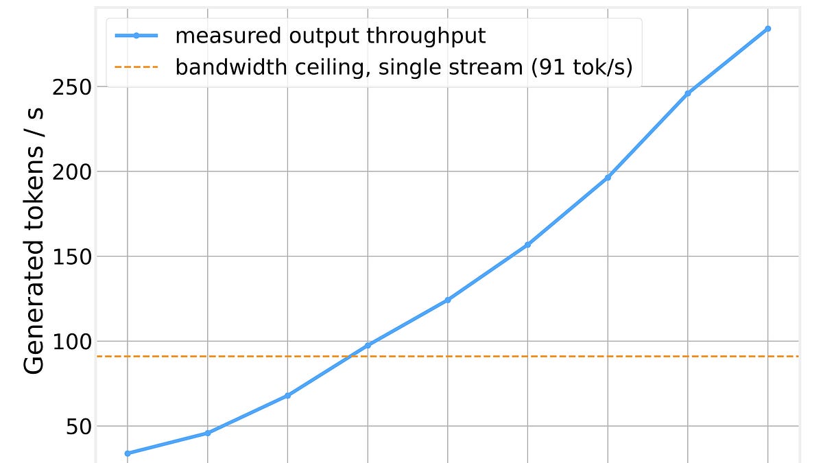
which helps keep output length relatively small. We test batch sizes between 1 and 256, doubling at each step, and measure the wall-clock time and number of output tokens, the throughput. We expect throughput to rise somewhat linearly with batch size until we hit the hardware limitations.
def run_batch(conversations, sampling):
    t0 = time.perf_counter()
    outs = llm.chat(conversations, sampling, chat_template_kwargs=NO_THINK, use_tqdm=False)
    elapsed = time.perf_counter() - t0
    n_gen = sum(len(o.outputs[0].token_ids) for o in outs)

    return outs, elapsed, n_gen

for batch_size in [1, 2, 4, 8, 16, 32, 64, 128, 256]:
    convs = [summary_messages(r) for r in works.iloc[:batch_size].itertuples()]
    _, seconds, n_gen = run_batch(convs, summary_sampling)
    print(f”batch {batch_size:4d}: {seconds:6.2f} s  {n_gen/seconds:6.1f} tok/s”)
The results are pretty clean:
Throughput increases steadily as the number of requests per batch increases. Starting with 34 tokens/s for single request and climbing to 284 tokens/s at the 256 requests level, well above the predicted 91 tokens/s ceiling. An 8x increase on the same model runnning on the same hardware. This result also provides an object lesson for harness design: whenever a step can be formulated as applying the same action to multiple inputs, its much more effective to do it as a single batch instead of as a tool call per item.
Since we are applying the same prompt, a literal example of single-instruction, multiple data, the KV tensors for the initial prompt are the same in every request. The PagedAttention block lets vLLM take advantage of this by caching them. This is known as automatic prefix caching and it means that long system prompts can cost less than you might expect when you’re able to take advantage of this caching mechanism.
During a cold run, the first time you run the model, 69% of prompt tokens come from the cache with the first request computing the share block that the remaining 255 requests can take advantage of. Running it again, a warm run, illustrates how all efficient this mechanism is. Practically nothing changes because all the caching benefits were already captured during the first run.
In total, out of 389k input tokens, only 120k were actually processed and wall-clock time is effectively the same across runs. Run time is dominated by output generation instead of processing the inputs. Caching saves computational power and memory bandwidth.
Structured outputs are a fundamental feature to successfully integrate the LLM output into a full featured pipeline. Typically, we ask the model to return its output as valid JSON but models don’t always cooperate. The model has to be integrated into harness that includes a parser, a validation step, and a retry loop.
vLLM makes our lives easier by providing a grammar-constrained decoding. It compiles a provided JSON pydantic schema and filters out any tokens that would result in an invalid output. We simply have to build a pydantic model class and provide it as an argument to the SamplingParams object that is consumed by the LLM class.
class PaperExtraction(BaseModel):
    scaling_domain: Literal[”machine_learning”, “physics”, “biology_ecology”,
                            “cities_society_economics”, “engineering_materials”,
                            “earth_climate”, “other”, “not_about_scaling”]
    quantity_scaled: str
    scaled_against: str
    is_empirical: bool
    claims_power_law: bool
    one_line_finding: str

schema = PaperExtraction.model_json_schema()

constrained = SamplingParams(
    temperature=0.0, max_tokens=300, seed=42,
    structured_outputs=StructuredOutputsParams(json=schema),
)
The schema in this example reflects the next step in our analysis. Our dataset was retrieved by searching for “scaling laws” and now we want to know what kind of scaling each paper is referring to, whether it is empirical or theoretical and wether it makes any claims about power-laws.
The entire dataset of 1,982 abstrcts was took in about 8 minutes, processed 1.35M input tokens at 2,820 tokens/s and 185k generated tokens at 384 tokens/s. Every output a valid python object that can easily be fed into our downstream analysis pipeline.
After the model is done processing the data, we are left with a nice clean set of results we can analyze. The first is to see how the distribution across fields changes over time. Physics gets the lion share with about 42% of the sample, with engineering and materials accounting for another third.
Now the question is, how well does Qwens classification based on simply reading the abstract match the original OpenAlex domain lables?
Overall, the results agree with the Physics classification matching most Physical Sciences papers, Biology and Ecology accounting for most of life science and Cities, Society and Economics having the majority of Social Sciences. The disagreements are also informative, with a significant fraction of Engineering Materials papers matching the Physical Sciences labels.
Next we look at how often a “scaling law” claim is actually refering to a power law, and is it an empirical or a theoretical claim?
The pattern is a good portrait of the various fields. Urban scaling is largely consituted by empirical power laws, the Bettencourt-West tradition. Physics claims power laws mostly based on theoretical approaches, such as dimensional analysis and renormalisation. Machine learning papers are mostly empirical but have a harder time claiming power laws, matching the literature’s drift from Kaplan-style fits toward broken and saturating curves. None of this information was in the original OpenAlex dataset. It all came from having an LLM reading 1,982 abstracts in less than 10 minutes on a desktop box.
So… which one one should you use, vLLM, or llama.cpp / Ollama?
The answer is… it depends. Their built for different workloads and the answer depends on the details of the job.
vLLM is NVIDIA CUDA centric and uses the Hugging Face safetensors format, with a plugin for GGUF support. It supports continuous batching over hundreds of requests with PagedAttention, automatic prompt caching, and structured outputs via token masking.
llama.cpp / Ollama is more focused on Apple Silicon but also supports CPU, CUDA, etc. It uses the self-described GGUF format that allow it to map weights directly to memory. Batching is supported as a fixed batch, and structured output can be generated using JSON schemas or GBNF grammar.
On my MacBook Pro, llama.cpp ran Gemma 3 1B in F16 at 118 tokens/s of generation for one user while on the DGX Spark, vLLM ran a 35B model at 34 tokens/s for one user and 284 tokens/s for 256 users at once. For individual requests, the Mac is faster but per CPU hour, the Spark did about eight times more work than its own single-stream number, and the Mac cannot do that trick: a laptop serving one chat has no reason to.
In my opinion, if you’re aiming for large scale processing, customizability, and have access to an nVidia GPU vLLM is the clear winner. Otherwise, llama.cpp / Ollama are the best choices. One more thing to keep in mind… vLLM is more flexible, but also more dangerous. vLLM’s features pay for the added complexity at scale, but at the price of a direct measurement to confirms it’s actually set correctly for your use case.
So far, we’ve done everything inside a single Python process. In production, we want to have our engine runing behind the usual OpenAI-compatible HTTP server. Fortunately, every argument we chose can be directly set in the command line. The vLLM equivalent of llama-server might look something like:
vllm serve Qwen/Qwen3.5-35B-A3B-FP8 \
    --max-model-len 4096 \
    --max-num-seqs 256 \
    --gpu-memory-utilization 0.50 \
    --limit-mm-per-prompt ‘{”image”: 0, “video”: 0}’ \
    --default-chat-template-kwargs ‘{”enable_thinking”: false}’ \
    --port 8000
After which you can just point any OpenAI compatible client to your endpoint and your pipeline can remain unchanged while benefiting from vLLMs advanced features.
If you enjoyed this post, consider subscribing and sharing it with a colleague who is about to run a model over a few thousand documents, and let me know in the comments which part of the inference stack you would like a deeper dive on next. The complete, runnable notebook is available in the series GitHub repository.
Don’t forget to
this post with others who might be interested, and encourage them to
so that they have access to the entire backlog of posts and be the first to know when a new a new article is posted.