Research Learning from experience is different from learning from curated datasets. Algorithms that learn from curated datasets can assume that all data is useful for learning. This is usually guaranteed by humans, who collect, clean, and filter raw data so that it is ready to be consumed by a learning algorithm. Experience, on the other hand, does not always contain learnable associations.
In most current applications of deep learning, our systems learn from human-curated datasets, and there has been little incentive for algorithm designers to develop algorithms that can learn from an unfiltered noisy data stream. The inability of existing algorithms to learn from experience is easy to demonstrate empirically with simple examples.
Imagine a simple data stream for learning a supervised prediction task. At every step, the agent observes a single binary-valued feature. If this feature has a value of one, then the ground-truth target is one. Otherwise, the ground-truth target is zero. The value of the feature is sampled from a Bernoulli distribution at every step; the probability of the feature being one is 1% at every time step.
We can visualize the input and target data stream for this task by looking at the values of the feature and target as a function of time. This is shown in Figure 1.
A linear system can learn this prediction perfectly by learning a weight of one from the feature to the prediction. A simple mechanism to learn this weight is to update the weight parameter with a small step-size parameter in the direction of the gradient computed with respect to the sample mean squared prediction error.
We can make this data stream more complex by adding some noise to the targets. Let's add either +1 or -1, randomly chosen, to the target at every step with a probability of 1%. The updated data stream is shown in Figure 2. Note that only a subset of the targets are predictable in this data stream—namely those that occur when the feature is one. The other +1 and -1 targets are unpredictable and thus unlearnable.
The second data stream is closer to experience than the first, because unfiltered experience has both predictable and unpredictable components. We can make the target more complex by adding noise to it. Let's add noise sampled from a normal distribution with zero mean and a variance of five (a different choice would give similar qualitative results). The targets for this updated data stream are shown in Figure 3. If we look at the targets now, it's no longer easy to find the predictable component from the noise by visual inspection.
So far, we have added noise to the targets. In raw experience, the inputs are also messier than our current single-feature input. Let's add 4095 more features that are part of the input data stream. Each of these features also samples its value from a Bernoulli distribution and has a 1% probability of being one. The difference between these features and the earlier feature is that these are uncorrelated with the target and useless for learning.
Now we can learn a linear predictor on this set of features using the noisy targets from Figure 3. Each feature has its own weight parameter connected to the prediction. All weights are initialized to zero. We learn using gradient descent combined with the SGD optimizer. The resulting predictions are shown in Figure 4.
A key observation to make here is that even though the only learnable aspect of the target is the +1 that occurs when the first feature has a value of one, this is not what SGD learns. SGD and its variants—such as Adam (Kingma & Ba, 2015) and RMSProp (Tieleman & Hinton, 2012)—try to minimize error on all targets and end up absorbing the noise. The reason for this is well understood: SGD assigns the credit for all prediction errors to all parameters with non-zero gradients, even if some of the parameters are connected to signals that are not useful for learning. It has no mechanism to differentiate targets that are predictable from targets that are not predictable and no mechanism to distribute the credit of an error to parameters more selectively.
We now switch to a different algorithm, called Incremental Delta Bar Delta, or IDBD for short (Sutton, 1992). Unlike SGD, IDBD can learn to assign a different amount of credit for a prediction error to different signals. In addition, IDBD can also learn not to distribute credit for a certain prediction error if the target is not predictable. We apply IDBD to the same problem and learn for the same number of steps and plot the predictions in Figure 5. Unlike SGD, IDBD only learns the predictable aspect of the data stream.
This same experiment can be reproduced in the non-linear case by extending IDBD to work with neural networks. We call the extension NetworkIDBD.
We need a data stream that requires non-linear feature learning. We construct one using the MNIST dataset (LeCun et al., 1998). The MNIST dataset has images of digits. Each image has a resolution of 28 x 28 and has an associated label.
We embed this image at the center of a larger 64 x 64 image. The center 28 x 28 pixels sometimes show an MNIST digit. The remaining pixels are once again noisy Bernoulli features and have a 1% probability of being one. Whenever a digit is rendered in the center, the target is either +1 if the digit is odd or -1 if the digit is even. When there is no digit in the center, the target is zero. At every step, there is a 10% chance that the input features will have a digit rendered in the center. Finally, we add noise sampled from a normal distribution with a mean of zero and a variance of five to the targets. We call this data stream NoisyMNIST. Samples from this stream are visualized in Figure 6.
The NoisyMNIST data stream, similar to the earlier data stream, has some targets that are predictable and some that are not predictable. Similarly, it has some input features that are correlated with targets (the center 28 x 28 features) and some that are not.
We connect these inputs to a hidden layer with 10,000 non-linear ReLU units. The weights from the inputs to ReLU units are sampled from the range (-0.0001, 0.0001) uniformly. The ReLU units are connected to the prediction unit with zero weights.
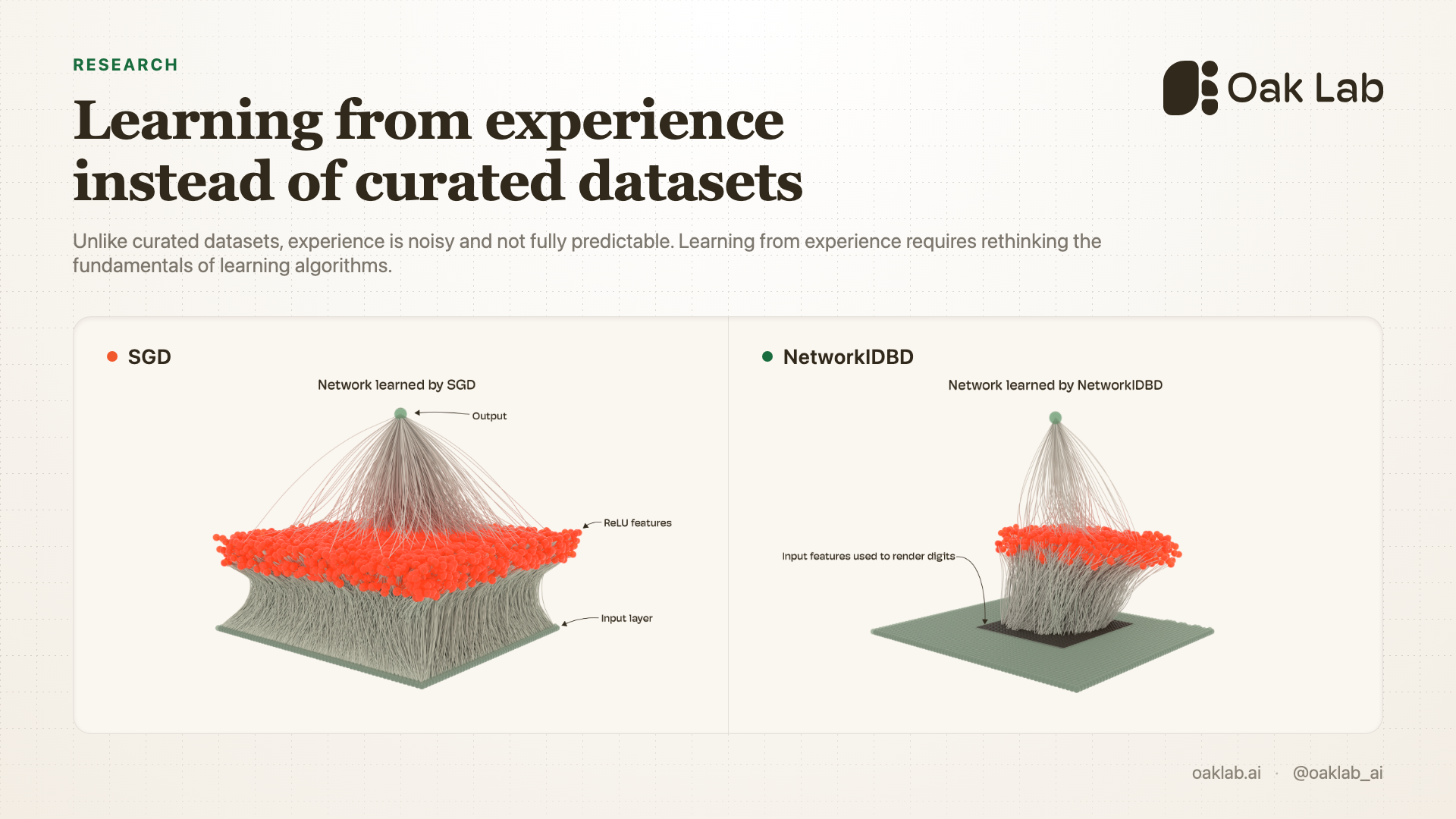
We learn the weight parameters using SGD and NetworkIDBD. After learning, we visualize which parameters of the network absorbed credit for learning this task by rendering all connections with a weight magnitude larger than 0.0002 (i.e., slightly larger than the largest initial value).
The network learned with SGD is visualized in Figure 7 whereas the network learned with NetworkIDBD is visualized in Figure 8.
The visualizations show that SGD increased the outgoing weights of all input features whereas NetworkIDBD learned by only increasing weights from the center 28 x 28 region (the region is highlighted in a different color), whereas SGD increased the weights of all features.
We believe that this limitation of SGD and its variants to try to learn all associations, even if they are just noisy, is a fundamental reason why current systems cannot learn well from noisy online data streams. To side step this limitation, current algorithms use large mini-batches that are sampled IID from the full dataset or a replay buffer. By averaging the gradients over many samples, they can reduce the impact of noisy associations on weight updates. However, this makes them a poor fit for online continual learning. To enable effective online learning from experience we have to build new algorithms that are better at credit assignment. Our bet is that the best methods would be those that learn to assign credit. NetworkIDBD is one instantiation of such algorithms.
References #
- Kingma, D. P., & Ba, J. (2015). Adam: A method for stochastic optimization. In Proceedings of the 3rd International Conference on Learning Representations. - Tieleman, T., & Hinton, G. (2012). RMSProp: Divide the gradient by a running average of its recent magnitude. COURSERA: Neural Networks for Machine Learning.
- LeCun, Y., Bottou, L., Bengio, Y., & Haffner, P. (1998). Gradient-based learning applied to document recognition. Proceedings of the IEEE. - Sutton, R. S. (1992). Adapting bias by gradient descent: An incremental version of delta-bar-delta. In Proceedings of the 10th National Conference on Artificial Intelligence.