A chatbot reply that lands in a couple of seconds hides hundreds of billions of matrix operations. Making an LLM run fast — and run cost-effectively — turns out to have surprisingly little to do with buying more GPUs, and everything to do with understanding where the time actually goes. This post walks through how much computation LLMs really need, how GPUs execute it, and the performance-engineering discipline that connects the two.
It helps to picture an AI system as five layers: the application layer, the middleware layer, the hardware layer, the network/storage layer, and the infrastructure layer. Here we focus on the middleware layer — the software that actually drives model execution — and work outward from there.
How much computation does an LLM actually need? #
To run LLM inference and training in a practical amount of time, you need a large-scale compute infrastructure built around GPUs. To see why, start with the raw arithmetic.
Inside a Transformer. When an LLM processes text, the input tokens are turned into vectors and passed through many Transformer blocks — the basic building unit of the model. Each block computes three intermediate representations (the query, key, and value) and uses them to perform attention, the step that decides which parts of the text to focus on. The result then flows through feed-forward stages such as output projection and SwiGLU, which reshape each token’s representation.
Almost all of this is matrix multiplication. Multiplying an m × k matrix by a k × n matrix takes roughly 2mnk floating-point operations, and an LLM repeats these multiplications in every layer. So the more parameters and layers a model has, the more rapidly the cost of processing a single token grows.
Take Llama 3 70B, a dense Transformer (one that uses essentially all of its parameters on every pass) with about 70 billion parameters. A useful rule of thumb is that generating one token costs about 2P operations, where P is the parameter count. That works out to 2 × 70 × 10⁹ = 1.4 × 10¹¹ — roughly 140 billion FLOPs for a single token, and about 140 trillion FLOPs for a 1,000-token answer. The reply feels instant, but a mountain of matrix math is churning underneath.
Why inference is stubbornly sequential. During inference, the model processes the prompt and then emits output tokens one at a time — and each new token feeds back in as input for the next. That dependency means generation can’t be fully parallelized. An inference server therefore has to do two things at once: crunch an enormous amount of math, and finish that work sequentially within the few seconds a user is willing to wait. That tension is what makes inference servers hard to design.
Why training is another order of magnitude. Inference only runs the forward pass with fixed weights. Training adds loss computation, backpropagation, gradient computation, and weight updates on top. To save memory, teams often use activation recomputation, which discards intermediate activations during the forward pass and recomputes the ones it needs during backprop.
A common estimate for total training cost is 6PT, where P is the parameter count and T is the number of training tokens; the factor of 6 rolls the forward pass, backprop, and gradient work into one number. Train Llama 3 70B on a trillion tokens and you get 6 × 70 × 10⁹ × 10¹² ≈ 4.2 × 10²³ FLOPs. Even a single GPU sustaining an effective 1 PFLOPS — that is, 10¹⁵ floating-point operations every second, continuously — would take more than ten years to finish. That’s why real training runs spread the work across hundreds to thousands of GPUs.
Put together: inference has to answer many users with low latency while doing billions of operations per token, and training has to chew through a workload larger by yet another order of magnitude. GPUs, which excel at running huge numbers of matrix operations in parallel, are the only practical answer. But a GPU doesn’t hand you performance for free — it comes with its own design philosophy, its own balance of compute versus memory bandwidth, and real communication costs once you use more than one.
Why GPUs — and why they don’t automatically deliver #
An LLM’s core operation, matrix multiplication, is the same multiply-accumulate repeated an enormous number of times. That’s a poor fit for a CPU, which spends its transistors on a few powerful, low-latency cores, and an excellent fit for a GPU, which spends them on many arithmetic units running the same operation in parallel.
A GPU keeps its control logic deliberately simple and pours most of its die area into arithmetic units. An NVIDIA H100 SXM, for example, packs 132 Streaming Multiprocessors (SMs), each with 128 CUDA Cores for general math and 4 Tensor Cores. The Tensor Cores are purpose-built for matrix multiplication and rip through the low-precision formats — FP16, BF16, FP8 — that dominate LLM work. The performance gap is stark: an H100 delivers 67 TFLOPS in FP32 and 989 TFLOPS on its FP16 Tensor Cores, versus a few TFLOPS for a typical server CPU. Given how much matrix math an LLM does, the choice makes itself.
The memory wall. High peak FLOPS don’t automatically translate into real throughput. A GPU runs thousands of threads at once and hides memory stalls by switching to another thread whenever one is waiting on data — but if you can’t feed the arithmetic units at all, they sit idle and throughput collapses. So memory bandwidth matters just as much as raw compute.
GPU memory is a hierarchy: registers (tiny and fastest, right next to the arithmetic units) → shared memory (fast, shared within an SM) → L2 cache (shared across the whole GPU) → HBM (the large, high-bandwidth main memory). An H100’s HBM offers 80 GB at 3.35 TB/s. The catch is that compute has outrun bandwidth. From the A100 to the H100, FP16 Tensor Core throughput jumped 3.2× (312 → 989 TFLOPS), but HBM bandwidth grew only 1.7× (2.0 → 3.35 TB/s). It’s now easy to end up with arithmetic units that are starved for data.
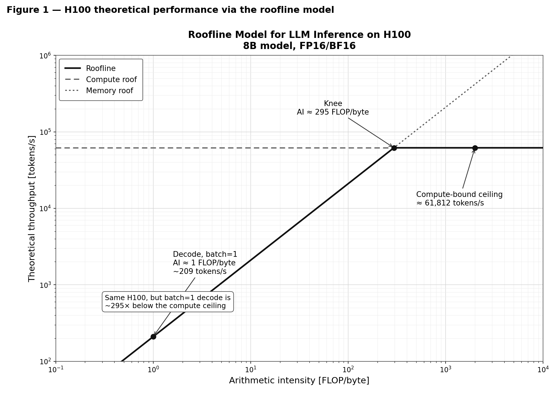
Whether a workload is compute-bound (limited by how fast the units can compute) or memory-bound (limited by how fast memory can feed them) comes down to arithmetic intensity — the amount of computation done per byte of data moved. A product of two large matrices has high arithmetic intensity and is compute-bound; a matrix–vector product (batch-size-1 inference) has extremely low arithmetic intensity and is firmly memory-bound. Plotted on a roofline model, everything left of the “knee” is capped by bandwidth and everything right of it by compute.
The gap this opens is dramatic. Running an 8B-class model on an H100 in FP16/BF16, the compute-bound ceiling works out to about 61,800 tokens/s, while a batch-size-1 decode is limited to roughly 209 tokens/s — about a 300× difference on the exact same hardware.
That single fact explains a huge amount of inference optimization. LLM inference splits into two phases: Prefill, which processes the whole prompt at once (highly parallel, GPU-friendly), and Decode, which emits tokens one at a time (serial, and bottlenecked on memory transfer rather than compute). Raising the batch size, or using continuous batching — dynamically re-forming batches as requests arrive and finish — pushes Decode’s arithmetic intensity up and out of the memory-bound regime. In other words, your software settings decide which regime the GPU runs in, and therefore what performance you can actually reach.
Scaling across many GPUs #
In production, GPUs come in servers, not singles — typically about eight GPUs per machine, a unit called a node. Eight GPUs give you 8× the raw performance in theory, but intra-node communication and synchronization overhead mean you never get a clean 8×.
Training is compute-hungry and pushes you to add GPUs. Large-scale continual pre-training — continuing to train from an existing model’s weights instead of starting over — routinely spans tens to hundreds of nodes. Get the parallelization or network layout wrong and communication, within and between nodes, becomes the bottleneck that leaves your GPUs half-idle. And because training has to stream the dataset continuously, storage throughput belongs on your watch list too.
Inference hits a different wall: when a model is too big to fit in one GPU’s memory, you’re forced across multiple GPUs. That opens up choices — splitting Prefill and Decode onto different GPUs, or tuning how aggressively you use the KV cache (which stores computed results for past tokens so they can be reused). Since memory capacity varies by GPU, you match the GPU type and count to the model. Squeeze out enough performance and you can even keep older GPUs in service for inference, which can meaningfully lower cost.
A reality check: most GPUs are badly underutilized #
Here’s the uncomfortable part: very few organizations get real performance out of their GPUs. In a 2024 AI Infrastructure Alliance/ClearML survey, only 7% of companies said their peak GPU utilization topped 85% — most sat at 51–70%. A Microsoft study of 706 GPU jobs found that in 85% of cases the system wasn’t delivering its available performance, thanks to mundane operational culprits: badly chosen batch sizes, preprocessing bottlenecks, checkpoint I/O stalls, and waiting on synchronization.
It’s also easy to misread the numbers. The “GPU Utilization” that nvidia-smi
reports is just the fraction of the last sampling interval in which at least one CUDA kernel was running — it says nothing about whether the whole SM array or the memory bandwidth is actually busy. So a reassuring-looking utilization figure can hide plenty of headroom in SM Activity or Memory Bandwidth Utilization. Finding the true bottleneck means reading several metrics together.
How to approach a performance problem #
Some of these problems live below the software line — in the GPU, the network, or the power and cooling. The engineering discipline for hitting and holding a system’s non-functional requirements (response time, throughput, scalability, resource efficiency) is performance engineering, and it runs on a simple loop: measure → analyze → implement → verify.
Its first commandment is don’t guess, measure. Rather than collecting data at random, you form a hypothesis and test it:
Baseline. Measure reference values — processing time, memory use, power draw — across several metrics.Profile. Use a profiler to watch the system’s internal behavior in detail.Hypothesize. From what the profiler shows, form a theory about the cause.Change one thing. Apply a single optimization at a time.Verify. Quantify the improvement against the baseline.
Amdahl’s law tells you where to aim. Speed up a stage that’s only 33% of total time by 100× and the whole system gets just 1.5× faster — so the first move is always to profile and find the parts that dominate the clock. It also pays to work top-down, from the latency you can see in the application and middleware layers down through the GPU, network, storage, power, and cooling. When the real cause is a lower layer, tweaking an upper one won’t save you.
In LLM inference and training, the stage that usually dominates is the model computation itself — which is exactly why the middleware layer that controls it is where most of the leverage lives.
Performance engineering in practice #
Running open models (weights and terms published, deployable in your own environment) or your own LLMs on a GPU cluster means splitting the work across GPUs, managing GPU memory, and controlling inter-GPU communication. On the training side, Megatron-LM and DeepSpeed handle this; for inference, vLLM and SGLang. Each exposes a set of performance-critical knobs — parallelization scheme, batch size, GPU-memory utilization, cache settings — that you tune to your model and hardware.
The parameter explosion. Training has a staggering configuration space. On top of a five-dimensional parallelization strategy — tensor, pipeline, data, context, and expert parallelism — you choose micro-batch size, global batch size, activation-recomputation granularity, and mixed precision (FP16/BF16/FP8). Worse, these interact. Raise tensor parallelism and you free memory to grow the batch, but you add communication that can drag throughput down. Turn on activation recomputation and you save memory but pay to recompute. The only reliable way to know the optimum is to measure — and a single trial can easily take hours. Inference has the same shape of problem: vLLM and SGLang expose CUDA-graph mode, batched-token limits, GPU-memory fraction, tensor-parallel degree, prefix caching, and more, and the best values shift substantially with each new GPU generation or model size.
You can’t tune what you can’t see. None of this works without measurement. Without a monitoring stack that continuously collects and visualizes metrics across the whole cluster, you can’t even name the bottleneck — let alone tell whether a change helped, whether a training job is thermally throttling, or whether storage I/O has become the limiter. A practical setup: an agent on every node exporting GPU utilization, SM Activity, memory, temperature, and power via NVIDIA DCGM Exporter, plus CPU, storage I/O, and network via Node Exporter; aggregate into ClickHouse and visualize with Grafana. (This is the same shape as the Performance Observability in Fixstars AIBooster.)
What performance engineering actually buys you #
To make this concrete, here are three cases from our own work (drawn from our book, AI Acceleration through Practical Performance Engineering).
443× faster inference — Llama 3-8B on H100. Starting from a naive 31 tokens/s with Hugging Face transformers
, we reached 13,739 tokens/s — a 443× gain. Cutting the GPU count from 8 to 1 removed pipeline bubbles (47 tokens/s). Applying FlashAttention-2 taught us a lesson: in a CPU-bound setup it can actually hurt. Batching brought us to 1,007 tokens/s, and the vLLM engine plus FP8 quantization finished at 13,739. The takeaways — “throwing GPUs at it doesn’t make it faster,” and “an optimization can backfire when the real limit is the CPU” — are invisible without measurement.
Pre-training in 1/9 the time — Llama 3-70B on H200. We cut the time to reach a target loss from 36 hours to 4 — a 9× reduction. The biggest lever was swapping the optimizer (SGD → Adam), which dropped the iterations to convergence from 1,800 to 300 (a sixth) at a mere 2% cost in compute throughput. Fixing convergence before chasing efficiency was the winning call.
Post-training in 1/6 the time — Llama-3.2-1B on A100. We took one epoch from 1,141 seconds to about 174 — 6.6× overall, in stages: removing a MemoryCallback (1.65×), automatic hyperparameter tuning that found tensor-parallel 4 → 1 (3.5×), Torch Compile (4×), and a larger global batch plus re-tuning (6.6×). A textbook case of “non-essential work had quietly become the bottleneck.”
Tuning training without burning your GPU budget #
Once you can measure, the hard question is how to find good settings within a fixed GPU budget — because the search itself burns GPU hours. Widening the search blindly is a trap: if searching costs more than the training time you save, you’ve lost money. Throw the whole parameter space at Bayesian optimization (which picks promising configs from past trials — Optuna is a well-known implementation) and post-training a Qwen3-Omni-30B-class model on 16 A100s can demand over 300 hours of search. Whether tuning pays off depends on the search time, the speedup you get, and how many times you’ll reuse the result. A three-month continual pre-training run can justify hundreds of search hours; a post-training job that finishes in hours cannot.
So the smart move is to fold in domain knowledge rather than lean on black-box search alone. Using memory- and communication-cost estimates to rule out obviously bad configurations and concentrate the search on promising regions gets you to good settings in far fewer trials. On the same Qwen3-Omni-30B post-training, a domain-knowledge search hit 1.52× over default in ~2 hours; combining domain knowledge with Bayesian optimization reached 1.79× in ~18 hours; and Bayesian optimization alone managed 1.70× — but took ~300 hours. The staged, knowledge-guided search beat pure black-box optimization on results and on time. (We drive this with a tuner called Zenith Tune in Fixstars AIBooster.)
Optimizing inference: pick the right metric first #
Inference optimization starts with deciding what to optimize, and users and operators care about different things. A user cares about end-to-end (E2E) latency — request in, full answer out — and about perceived speed while the answer streams, measured as tokens/s/user. The operator paying for the hardware cares about tokens/s/GPU: how much a single GPU can produce.
The trap is that these pull against each other. Batch more requests together and tokens/s/GPU climbs — but requests wait longer in the queue and E2E latency gets worse. Over-optimize per-user speed and GPU efficiency drops and your costs rise. The real question in production is: where’s the operating point that maximizes GPU efficiency while still honoring the user experience? You express the experience as SLAs — “E2E latency under X,” “at least 20 tokens/s per user” — and search for the most efficient settings inside that envelope.
The vLLM team and NVIDIA made the same point in their gpt-oss-120B work: maximizing any single metric isn’t enough; what matters is pushing up the whole throughput-vs-latency Pareto frontier (the line where improving one necessarily worsens the other). Concretely, you auto-search the inference engine’s parameters while sweeping concurrency and request rate, measuring E2E latency, generation speed, and GPU efficiency, and keep the operating point that maximizes efficiency within the SLA.
Tuning gpt-oss-120B this way (H100 × 8) with AIBooster shifted the entire Pareto frontier upward versus vLLM’s recommended settings — and in the mid-load range (128 concurrent connections) throughput rose 21% and per-user generation speed rose 30%.
Cloud or on-premises? #
There are two broad ways to get GPU infrastructure, and neither wins outright — the right call depends on workload, time horizon, cost, and security.
Cloud lets you start immediately and pay for exactly what you use, which suits short experiments, spiky inference traffic, and trying out a new GPU generation. Run it hard for the long haul, though, and costs mount — while data sovereignty and network latency can become real constraints.
On-premises demands upfront capital and an operations team, but it’s usually more cost-efficient over the long term and lets you tune network and storage to your workload. Crucially, it keeps AI processing entirely inside your own environment, so sensitive data never leaves the building.
That last point is what makes on-prem compelling for local LLMs — running open models like Llama or Qwen in house. Closed cloud models (weights unpublished, reached through an API or managed service) are powerful and convenient, but plenty of organizations can’t send confidential source code or internal documents to a third party. For a programming workflow, the real question becomes how close you can get to that closed-model experience — code generation, code review, internal document search, RAG (Retrieval-Augmented Generation: searching your own documents and generating answers grounded in the results) — entirely inside a secure local environment.
On-prem scales, too. For a team or a small deployment, a GPU workstation with a chat UI, coding assistance, an agent runtime, and monitoring may be plenty — the kind of stack packaged in products like Fixstars AIStation. Go bigger and you’re into data-center territory: multiple GPU servers, with the number of GPUs, network, storage, power, and cooling all designed together. A purpose-built facility is a long, expensive project — and keeping pace with GPU generations is its own challenge — which is why container-type data centers have become a popular middle ground between a single workstation and a full building.
The takeaway #
The point worth carrying away is that GPU performance is never decided by software alone. The settings on an inference engine or training framework can move the needle enormously — but only on top of a healthy foundation of GPU servers, network, storage, power, and cooling. To get AI performance reliably, you have to stop treating software, hardware, and infrastructure as separate concerns and start treating them as one system. Measure first, work top-down, change one thing at a time — and let the numbers, not your intuition, tell you where the time is going.
References #
- Grattafiori, A. et al. “The Llama 3 Herd of Models.” arXiv:2407.21783, 2024.
- Kaplan, J. et al. “Scaling Laws for Neural Language Models.” arXiv:2001.08361, 2020.
- Williams, S. et al. “Roofline: An Insightful Visual Performance Model for Multicore Architectures.” Communications of the ACM, 52(4), 2009. doi:10.1145/1498765.1498785.
- Dao, T. “FlashAttention-2: Faster Attention with Better Parallelism and Work Partitioning.” arXiv:2307.08691, 2023.
- AI Infrastructure Alliance / ClearML. “The State of AI Infrastructure at Scale 2024.” 2024.
- Gao, Y. et al. “An Empirical Study on Low GPU Utilization of Deep Learning Jobs.” ICSE ’24, ACM, 2024. doi:10.1145/3597503.3639232.
- vLLM Team & NVIDIA. “GPT-OSS 120B: Optimizing Large Model Inference.” vLLM Blog, 2026.