In early 2026, a startup called Taalas launched the HC1 chip, delivering reported inference speeds of 17,000 tokens/second on LLaMA 3.1 8B[1]. Its core innovation is: physically embed the model weights into the chip itself, eliminating memory bandwidth as a bottleneck. By design, base model weights are physically fixed at fabrication — runtime adaptability comes through LoRA, and model updates through a new mask cycle. Taalas has publicly stated that adapting to a new model requires changing only two custom metal interconnect layers[2]. From there, I treat those public specs as constraints and reverse-engineer HC1's architecture, performance, and economics — deriving internal parameters from first principles, quantifying the key metrics, and being explicit about every assumption and uncertainty range along the way.
A note on precision: Derived values (e.g. 941 Mbit/layer) reflect the math, not false precision. Aggregate uncertainty is ±20–30%; treat the constraint ranges in the body as authoritative.
- Pipeline architecture, F=1 (fold factor) : Each of the 32 Transformer layers has its own dedicated PE array — the structural prerequisite for 17k tok/s, at the cost of a non-compressible die area
- PE count : Reference solution 4,096 PE/layer @ 942 MHz; feasible range 2,600–4,900 PE/layer @ 800–1,500 MHz
- Weight ROM precision : 3–6 bit mixed quantization is the only feasible range under via density, yield, and lithography constraints; INT4-equivalent reduces via count to 1/4 of FP16
- KV-cache concurrency ceiling : INT8 ceiling of4–5 users
- **LoRA SRAM** : Rank-16 adapter, FP16 ~15 mm², INT8 ~7 mm²; shares on-chip budget with KV-cache
- **Performance** : HC1 Wₜₒₜₐₗ ≈**180 ms** vs. H200 ≈**2,204 ms** (**~12×** faster; 1k-token prompt, N=4 users)
- Economics : Mask-only NRE is 2–3 orders of magnitude below full tape-out; no HBM at inference. The 815 mm² die is H100-scale — not a "small chip, low cost" story
For context: H200 delivers roughly 230 tok/s, Groq around 600 tok/s, Cerebras around 2,000 tok/s[3]. At 17,000 tok/s — equivalent to approximately 13,000 English words per second, or 2,000 lines of Python code per second — output is effectively instantaneous for a single user. The speed matters in two practical scenarios: cloud inference services (shorter completion times mean faster slot turnover, more requests served per unit time), and agentic workflows (chained calls require massive token generation in milliseconds).
1.1 The core idea: eliminating the memory bandwidth wall #
Traditional GPUs running LLM inference face a fundamental tension: generating each token requires the entire model's weights from HBM into compute units. For LLaMA 3.1 8B — approximately 6.7B parameters, roughly 3.4 GB at INT4 — that's a full weight transfer per output token. The bandwidth bottleneck becomes the hard ceiling on throughput, regardless of how much compute is available.
Taalas's solution: burn the weights into the chip, so inference reads them directly instead of moving them.
Taalas has disclosed limited detail on the specific implementation. Based on their public description — "only two custom metal interconnect layers need to be changed to adapt to a new model"[2] — the most natural standard CMOS realization is Via ROM: weights are encoded in the top metal layers by the presence or absence of vias (vertical conductors). A via present = bit 1; via absent = bit 0. The weight pattern is written at fabrication time through custom masks and locked in permanently. Weights connect directly to compute units through hardwired paths, with no address decoding, cache misses, or bandwidth limits. Via ROM is our inference about the specific implementation — it is not Taalas's official terminology.
The tradeoff is immutability: the base model is physically frozen in the via layer, and a given chip runs only LLaMA 3.1 8B. Adapting to a new model requires new custom mask layers (~two-month cycle, see §5.1); Taalas supports LoRA adapters for limited runtime adaptability[5].
1.2 Chip cross-section: ROM layer above, transistors below #
HC1 makes more sense once you see what it actually looks like in cross-section.
Figure 1: HC1 chip vertical cross-section
From bottom to top, three distinct physical layers:
- Green (bottom) : The transistor layer — 53B transistors, determines the 815 mm² die area. All compute, memory, and I/O live here. Transistors tile horizontally; vertical stacking is not possible.
- Blue (middle) : Standard BEOL metal routing for signal interconnects and power distribution.
- Gold (top) : Two custom metal interconnect layers added by Taalas[2], where via presence or absence encodes each weight bit.
The ROM layers share the same horizontal footprint as the transistor layer — they sit on top like a laminate, adding no die area. The 815 mm² is set entirely by the transistor layer. That's the structural underpinning of the entire cost story: 32 independent copies of the weight ROM come at zero die area cost.
The lithography specification for the two custom masks is not publicly disclosed. Back-calculating from an INT4 via pitch of approximately 226 nm, the required precision falls within KrF (248 nm) lithography[7]. A single KrF mask costs roughly $5,000–$15,000; two masks run approximately $10,000–$30,000. Compare this to a full N6 mask set (75+ layers, ArF immersion lithography) at approximately $5M–$15M[8] — a difference of 2–3 orders of magnitude.
1.3 All 32 layers unrolled: why F=1 #
HC1 targets LLaMA 3.1 8B, which has 32 Transformer layers. The defining architectural decision is Fold Factor F=1.
What is the fold factor? It determines how many layers share a single physical compute unit (PE array). F=1 means each layer has its own dedicated PE array; all 32 layers form a 32-stage pipeline operating concurrently. F=32 means one shared PE array that 32 layers time-multiplex, cutting throughput by 32×. Critically, via ROM is physically fixed — regardless of F, all 32 layers' weights must remain on-chip. The ROM itself cannot be folded.
Figure 2: Fold Factor F=1 vs. F=32 F=32 could theoretically consolidate 32 dedicated PE arrays into a single shared array, but the via ROM — with all 32 layers' weights — must remain complete. The area savings from folding are limited to the PE arrays themselves (~2.2 mm²), negligible against an 815 mm² die, while the throughput penalty is the full 32× (17,000 → 531 tok/s). In a via ROM architecture, F>1 delivers almost no area benefit while sacrificing throughput entirely. F=1 is the only sensible choice: the 32 ROM copies cost nothing (ROM layers sit above the transistor layer and add no die area), and the "cost" (32 dedicated PE arrays) turns out to be the smallest component of the die.
1.4 PE count and clock frequency #
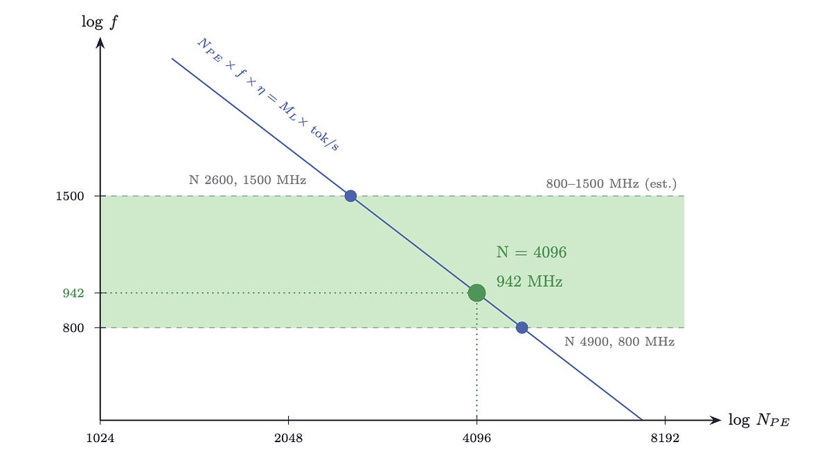
Once the throughput target is fixed, PE count and clock frequency are not directly observable — they're jointly constrained, sitting on the same hyperbola. Pinning the design point requires an independent engineering boundary to narrow the feasible region.
Given a target of 17,000 tok/s, PE count per layer (N(PE)) and clock frequency (f) satisfy the throughput constraint (Eq. 1; where Mₗ = 226.5M MACs/layer is the per-layer compute for LLaMA 8B, and η ≈ 1 is pipeline efficiency under F=1 full unrolling):
Equation 1 traces a hyperbola: more PEs means lower required frequency, and vice versa. The throughput target alone cannot uniquely determine a design point — we need an independent constraint on frequency. For compute arrays at the 815 mm² scale, combining long-wire delay and power density, a practical engineering frequency range is approximately 800–1,500 MHz[4]. (N6 process supports much higher frequencies for optimized designs, but timing closure and thermal density typically constrain large NPU arrays to this band.) The two intersections of this frequency range with the hyperbola bound the feasible PE count (Figure 3):
Figure 3: PE count vs. clock frequency design space
The two intersection points bound the feasible range: the 1,500 MHz upper bound corresponds to N(PE) ≈ 2,600; the 800 MHz lower bound to N(PE) ≈ 4,900. There is no unique solution — the feasible PE count spans roughly 2,600–4,900.
N(PE) = 4,096 PE/layer @ 942 MHz sits in the middle of this range — a convenient reference point (64 × 64 = 4,096), which validates to 17,001 tok/s against the official 17,000 (error: 0.006%). HC1 is not a systolic array; the PE array need not be square. 4,096 is a clean power of two, not an architectural necessity. The actual engineering design point could be anywhere in the feasible range; we use 4,096 PE/layer as our analysis baseline throughout.
With F=1, each of the 32 layers instantiates independently. Total on-chip PE count: 4,096 × 32 = 131,072.
1.5 How ROM weights feed into PEs at speed #
Under F=1, the chip contains 32 fully independent compute blocks, each dedicated to one layer. Each block operates identically: an activation vector flows in from the preceding layer, weights from the dedicated ROM are read out column by column through sense amplifiers, and the two are multiplied and accumulated in the PE array, with output passing to the next stage. Figure 4 shows the complete datapath:
Figure 4: Single compute block datapath
The "hardwired path / zero access latency" indicator on the left of Figure 4 is the core performance mechanism. In a GPU, generating each token requires all model weights from HBM — incurring hundreds of nanoseconds of memory access latency and consuming enormous bandwidth. This is the fundamental bottleneck for GPU LLM inference. In HC1, weights are encoded as via presence or absence and permanently wired to the PE array; every cycle begins with weights already present, requiring no address calculation, cache lookup, or bus transfer. Access latency is zero. Bandwidth is no longer the limiting factor. Compute utilization can now approach what's actually possible when the memory wall isn't in the way.
Each PE reads one INT4 weight per cycle through sense amplifiers (SA) — circuits that detect minute current differences on via lines to determine whether a via is present. SAs store nothing; they only detect. But they exist in very large numbers, making them the largest unknown in the die area budget.
Under F=1, the layer-select MUX present in F=32 (Figure 2, right) is eliminated, along with the full row address decoder (replaced by a simple sequential counter). The sense amplifiers themselves remain unavoidable.
2.1 Area distribution overview #
The methodology: anchor the components derivable from process specifications and public interface standards; work forward from physical constraints (parameter count × quantization precision → SA column count → SA area) to derive the major unknowns; then conservatively bound the remainder. Confidence decreases across the four components: fixed known items have hard boundaries; SA/ROM is derived from architectural constraints but carries process density uncertainty; KV SRAM is the residual after SA/ROM is determined, inheriting that uncertainty; undisclosed IP can only be upper-bounded.
Figure 5: HC1 area distribution
The components are causally linked: quantization precision fixes the via count → locks SA column count and SA area → constrains available KV SRAM → sets the concurrency ceiling. In numbers: PE arrays ~2–6 mm² (<1%, sector enlarged in figure); fixed known items ~140 mm² (17.2%); SA/ROM ~230 mm² (28.2%, midpoint); undisclosed IP ~100 mm² (12.3%); KV-cache SRAM ~349 mm² (42.8%, midpoint). The sections below work through this causal chain in order.
2.2 Quantization precision: a triple-constraint analysis #
According to media reports[5], HC1 uses a custom 3-bit + 6-bit mixed quantization: 3-bit as the base data type, with some parameters elevated to 6-bit. The weighted average is approximately 4.5 bits, corresponding to roughly 36 Gbit of total vias. We use the 4.5-bit average as the primary baseline and INT4 (4-bit) as a standard reference; qualitative conclusions are consistent across both for the following three constraints.
Weight quantization precision doesn't just determine model accuracy — it simultaneously fixes three physical properties: total via count, lithography cost, and manufacturing yield. The critical via pitch follows from die area and total via count (Eq. 2):
where A(die) = 815 mm², N(bits) is the total weight via count, and the factor of 2 accounts for the two custom metal layers. Substituting HC1’s actual values (4.5 bit, ~8B parameters): √(2 × 815 / 36×10⁹) mm = 213 nm.
Table 1: Quantization Precision vs. Via Pitch, Yield, and Lithography Cost
Both 4.5-bit (213 nm) and INT4 (226 nm) fall within KrF (248 nm) lithography[7]. This is where the three constraints converge into a single feasible region:
- FP16 : Requires via pitch ≤ 123 nm — ArF immersion lithography, costing hundreds of millions of dollars in equipment, fundamentally incompatible with the "two low-cost masks" business premise
- INT8 and above : Pitch tightens to ≤ 174 nm; lithography costs rise significantly, yield risk worsens
- The 3–6 bit mixed range (~213–261 nm pitch) : Lands squarely within KrF (248 nm) lithography, self-consistent with the "two low-cost custom masks" economics
HC1's precision choice is not coincidental — it is the intersection of three independent constraints. Taalas has publicly stated that HC2 will move to standard 4-bit floating-point formats to improve model accuracy[5].
2.3 ROM readout circuits and sense amplifiers #
SA area is jointly determined by three inputs: LLaMA 8B parameter count (public), HC1 quantization precision (~4.5 bit, sourced above), and 4,096 PE/layer (our analysis baseline).
Step-by-step derivation: The 32 Transformer layers share identical architecture (hidden dim 4,096, FFN 14,336), so weight volume is equal per layer. Distributing 941 Mbit across 4,096 PE/layer gives ~230K bits per PE, corresponding to a sub-array of √230K ≈ 479 columns. One sense amplifier per column at approximately 100 transistors per SA:
Adding row drivers, data paths, and fanout buffers (~10–25B transistors) gives 18–34B total transistors. Converting at TSMC N6 HD logic density (ρ(HD) ≈ 110 MT/mm²):
Midpoint estimate: ~230 mm². High-end estimate: ~300 mm². These bracket the SA/ROM segment in Figure 5.
2.4 PE Array #
Single-PE area is estimated from transistor counts for each sub-circuit. An INT4 weight × INT8 activation MAC (with 20-bit accumulator):
Table 2: Single PE Transistor Count Estimate
TSMC N6 HD logic density ~113 MT/mm² (0.0088 μm²/T), with routing overhead (~1.7×): Total for 4,096 PE/layer × 32 layers: ~2.2 mm². Including global interconnect and control logic worst case: ~3–6 mm², or ~0.3% of die area. The marginal cost of compute is effectively zero.
2.5 Fixed Known Items #
Two components independently derivable from public information:
Table 3: Fixed Known Items Area Estimate
PCIe specification (Gen4 x16) is inferred; Taalas has not publicly disclosed it. The 2×100GbE interfaces are confirmed by two visible QSFP28 cages on the board[1].
2.6 Undisclosed IP #
Attention compute and other nonlinear operator hardware are very small (~1–3 mm² total across 32 layers). Remaining undisclosed circuitry is conservatively bounded at ~100 mm² (LoRA SRAM, ECC logic, and global interconnect included). We keep this as a single bucket so that LoRA SRAM and KV-cache SRAM can each be sized independently in §2.7 and §2.8.
2.7 LoRA SRAM area #
Taalas supports LoRA adapters[5]; adapter weights require dedicated on-chip SRAM. Rank and scope are not publicly disclosed; we use a common inference deployment configuration (rank 16, covering all attention matrices Q/K/V/O)[9].
LoRA adds low-rank matrices to each target weight matrix W — A ∈ ℝ^(r × dᵢₙ) and B ∈ ℝ^(dₒᵤₜ × r) — adding r(dᵢₙ + dₒᵤₜ) parameters per target. Summing across all four matrices for all L layers and multiplying by bit width:
Q and O share the full hidden dimension (d(QO) = 4,096); K and V share the GQA key-value dimension (dₖᵥ = 1,024). For LLaMA 3.1 8B:

**Table 4: Per-Layer Q/K/V/O LoRA Parameters (r = 16)**
K/V have dₒ = 1,024 because GQA uses only 8 KV heads (8 × 128), vs. 4,096 for Q/O. Total across 32 layers: ~13.6M parameters. SRAM area at macro-level density (ρ(macro) = 0.067 μm²/bit, including SA/decoder/ECC overhead):
Table 5: LoRA SRAM Area Estimate
2.8 KV-cache SRAM area #
KV-cache holds dynamically generated intermediate data at inference time and must reside in SRAM (via ROM is read-only and cannot hold runtime state). KV-cache precision is independent of weight precision — HC1's 3–6 bit quantization applies only to hardwired weights; KV-cache typically stays at FP16 or INT8, as dynamic activations are more sensitive to quantization error. In short: the model needs to retain the K and V attention matrices for all preceding tokens to generate coherent continuation — this memory grows linearly with both user count and context length.
Two steps to derive per-user area:
Step 1: per-user KV buffer bit count
Substituting LLaMA 3.1 8B parameters (GQA, tₘₐₓ=2,048, L=32, nₖᵥ=8, d(head)=128): FP16 (B(prec)=16 bit) gives ~2 Gbit/user (256 MB); INT8 gives ~1 Gbit. Where tₘₐₓ=2,048 is a deployment assumption aligned with Taalas's published benchmark condition ("Input 1k / Output 1k"); the context window is configurable, and larger values linearly increase per-user KV area.
Step 2: per-user KV buffer macro area
At macro-level density ρ(macro) = 0.067 μm²/bit (including SA/decoder/ECC overhead): FP16 per user ~143 mm², INT8 ~** 72 mm²**.
Step 3: total KV SRAM for N concurrent users
Available KV-cache area = total die area minus all other allocated components. Subtracting LoRA worst case (§2.7, FP16 ~15 mm²), with remaining Other IP = 100 − 15 = 85 mm²:
- At SA midpoint (~340 mm² available): FP16 ~2 users, INT8 ~4–5 users
- At SA high estimate (~270 mm² available): FP16 ~1–2 users, INT8 ~3–4 users
This is far below GPU concurrency (H200 comfortably handles dozens to hundreds of concurrent users). But this doesn't undercut the throughput advantage: at 17k tok/s, per-user completion time W compresses to roughly 118 ms, and slot turnover runs approximately 18× faster than H200 INT8 — net requests completed per unit time is actually higher. Context length, concurrency, and KV quantization precision form a three-way tradeoff on a fixed SRAM budget: increasing any one compresses the other two. The full picture follows in §3.
3.1 Why not tok/s? #
Operators pay for time (chip lease, power, ops) and earn from completed requests. So the right metric is requests completed per unit time (λ), not tok/s — tok/s is just one input: faster tok/s → shorter per-request completion time W → higher λ.
§2.8 determined HC1's concurrency ceiling (N=4–5, INT8 midpoint). This feeds directly into W. Little's Law[10] gives the three-way relationship:
Under lockstep decode (the chip generates one token per step for all N users simultaneously), decode-phase completion time is:
Note that lockstep decode is structurally different from GPU continuous batching — all N users advance in the same pipeline cycle, with no dynamic scheduling or request queuing.
Figure 6 makes this intuitive: given equal concurrency N, the chip with smaller W completes more requests in the same time window — higher λ.
Figure 6: Little's Law — smaller W means more requests completed per unit time
The full W calculation also requires time-to-first-token (TTFT); see §3.2.

## 3.2 Time-to-first-token (TTFT) and its impact on W
Equation 13 covers only the decode phase. The total user-perceived wait time is:
TTFT is the time to complete prompt prefill and emit the first output token. The two chips have different prefill architectures:
- HC1 : The via ROM pipeline shares the same PE array for prefill and decode; prefill throughput is approximately equal to decode, ~17,000 tok/s
- H200 : Compute-bound prefill — the entire prompt can be batch-processed as a matrix operation, approximately 33,000 tok/s (estimated midpoint, not measured)
Substituting into Eq. 13 and Eq. 14 (N=4, L<sub>resp</sub>=500, 1k-token prompt): Table 6: HC1 vs. H200 completion time
HC1 is 18× faster in decode alone. Including TTFT, total completion time for a 1k-token prompt is ~12× faster. TTFT accounts for 34% of HC1's total time (62/180), compared to under 2% for H200 (30/2,204) — prefill latency is HC1's current structural weak point.
With longer prompts, HC1's TTFT grows faster (17k tok/s prefill vs. H200's ~33k tok/s), narrowing the gap: at 4k tokens the advantage is approximately 6×. The full prompt-length sweep follows.
3.3 Full prompt-length comparison #
HC1 starts low (small W(decode)) but rises steeply (slow prefill); H200 starts high (large W(decode)) but rises shallowly (fast prefill). The H200 prefill rate is an estimate (~33k tok/s); if the actual range is 20k–60k tok/s, the crossover falls between 46k and 113k tokens.
Figure 7: W_total vs. prompt length (TTFT + decode, N=4) Across typical operating conditions (1k–8k prompt tokens), HC1's total completion time stays below one-tenth of H200's. The crossover is at approximately 72k tokens — beyond the practical range of virtually all conversational inference workloads. For API providers, faster slot turnover and sub-200ms response times carry clear value in latency-sensitive applications: real-time assistants, code completion, and multi-step agentic workflows.
HC1's die area (815 mm²) is nearly identical to the H100 GH100 (814 mm²)[6]. This is not a "small chip, low cost" argument. The cost advantage comes from two independent sources:
4.1 Low NRE, fast iteration #
Each model update requires new custom masks for only two layers — tens of thousands of dollars, roughly two months out. Full N6 tape-out runs $5M–$15M. That's 2–3 orders of magnitude cheaper per iteration.
4.2 No HBM packaging #
HBM is a major cost center for high-end GPUs (H100's HBM3 packaging is estimated at 30–40% of total card cost). HC1 weights are fixed in via ROM; inference requires no HBM at all. That cost line is absent from the BOM entirely.
Via ROM's extreme specialization is what makes HC1 fast — and what defines its engineering boundaries. The three design considerations below all trace back to the same root decision: weights are physically permanent.
5.1 Risk 1: model iteration #
Each new frontier model release represents an adaptation cycle for HC1. The key question is what "two months" actually means in practice.
What "two months" covers
Taalas's claim refers to the cycle from finalized new model weights to first-wafer-out: custom via pattern GDS verification, two-layer mask fabrication (~1–2 weeks per layer), and TSMC N6 wafer fab cycle (~6–8 weeks standard).
What "two months" does not cover
Model training and accuracy validation (assumed external); back-end packaging and burn-in; customer qualification and acceptance; and production ramp from engineering samples to delivery volume. The end-to-end cycle from "decide to switch models" to "available at scale" likely adds 1–2 months conservatively.
Foundry scheduling is the hidden variable
TSMC N6 capacity is persistently tight; advance booking typically requires securing wafer slots months ahead. "Two months" holds only if foundry capacity is pre-reserved. A sudden competitive release requiring an immediate response is constrained by queue position, not Taalas's internal design speed. Hot-lot fast-track can compress wafer cycle to 3–4 weeks but carries significantly higher cost and is not the default.
For planned updates with pre-reserved foundry slots, "two months" is a reasonable estimate. For reactive responses to sudden competitive pressure, the practical window may extend to 4–6 months — during which a newer model may gain market share ahead of the updated chip arriving.
5.2 Risk 2: manufacturing yield #
Fabrication defects in via ROM — missing or shorted vias — map directly to weight bit errors with no software correction path. At 32 Gbit of total via count, yield management is a non-trivial engineering problem. INT4 quantization reduces the via count to approximately 1/4 of FP16, providing meaningful yield headroom. No yield data has been publicly disclosed.
5.3 Risk 3: scale ceiling #
At 815 mm², HC1 is approaching the reticle exposure limit for a single die. LLaMA 70B would require approximately 3 TB of via ROM — far beyond single-die capacity. Scaling to larger models requires a chiplet approach, with corresponding increases in interconnect design complexity.
HC1 makes a credible case that via ROM is a viable path to competitive inference economics: the performance gap over GPU inference is real, the cost structure is differentiated, and per-model iteration is operationally practical at mask-only NRE. The concurrency ceiling, prefill latency at long context, and model iteration window are well-characterized tradeoffs — not unknowns — and they define the design space HC2 works within.
Taalas has put a genuinely interesting chip in front of the industry. The HC1 is worth studying not just for what it achieves, but for how cleanly the architecture maps to its constraints — that kind of design discipline is rarer than it sounds, and it gives the whole field a useful reference point for what purpose-built inference silicon can look like.
Data sources: Taalas official product page and third-party media reports (company claims, not independently verified).
References
- Taalas. “HC1 Technology Demonstrator.” taalas.com , February 2026. taalas.com/products/
- Freund, K. “Taalas Launches Hardcore Chip With ‘Insane’ AI Inference Performance.” Forbes , February 19, 2026.
- NVIDIA. “Deep Learning Performance — AI Inference.” NVIDIA Developer , February 2026. developer.nvidia.com/deep-learning-performance-training-inference. Artificial Analysis. “Llama 3.1 8B Instruct — Provider Speed Benchmarks.”Artificial Analysis , accessed March 2026. artificialanalysis.ai.
- Engineering estimate based on published operating parameters of large-area AI accelerator arrays, including Groq TSP and Cerebras WSE. No official TSMC N6 specification is available for this parameter.
- AlphaSignal. “Taalas AI Chip: 17,000 tokens/sec beats Nvidia by 74x.” LinkedIn Pulse , March 2026. linkedin.com/pulse/taalas-ai-chip-17000-tokenssec-beats-nvidia-74x-alphasignal-uozoc/
- TechPowerUp. “NVIDIA H100 SXM5 80 GB.” TechPowerUp GPU Database , accessed February 2026. techpowerup.com/gpu-specs/h100-sxm5-80-gb.c3838.
- ASML N.V. “ASML Ships 1,000th KrF Lithography System.” ASML , April 22, 2008. asml.com/en/news/press-releases/2008/asml-ships-1000th-krf-lithography-system.
- Hughes, G. et al. “Mask and Wafer Cost of Ownership (COO) from 65 to 22 nm Half-Pitch Nodes.” Proceedings of SPIE , vol. 7028, 2008. doi:10.1117/12.793067.
- Hu, E. J. et al. “LoRA: Low-Rank Adaptation of Large Language Models.” ICLR , 2022. arXiv:2106.09685.
- Little, J. D. C. “A Proof for the Queuing Formula: L = λW.” Operations Research , vol. 9, no. 3, pp. 383–387, 1961. doi:10.1287/opre.9.3.383.