LLMs have every English word in their vocabulary, but some of those words may never appear in their output. LLM-generated text is measurably less lexically diverse than human writing. The researchers at GING set out to investigate one possible reason why an LLM might never produce a specific word, even if it is appropriate for a given context.
When an LLM predicts the next token, it reads the preceding context and produces a logit for every token in its vocabulary. A token can be a whole word, a piece of a word, punctuation, a space, or any other text fragment. For example, Llama 3 has a vocabulary of 128,256 possible tokens. When inferring the next token, each of these options is assigned a logit.
The logit isn’t a probability but a raw numerical score. A function called softmax turns the logits into probabilities by raising the mathematical constant e to the power of each logit, then dividing that value by the sum of all the exponentiated logits.
i= e
logitΣ
ije
logit
j Softmax scales based on the raw numerical gap between two numbers, not their ratio. For example, 4:2 and 2:1 represent the same ratio, but the absolute gaps are different: 4 - 2 = 2, while 2 - 1 = 1.
- Applying softmax to [4, 2] gives approximately**[0.881, 0.119]. - Applying softmax to [2, 1] gives approximately[0.731, 0.269]**.
Even though the ratios are identical, the larger absolute gap makes the higher value much more dominant after softmax is applied.
Temperature #
Temperature is a variable adjusted during inference, usually treated as a creativity parameter. Increasing the temperature makes the output more varied, while decreasing it makes the model's outputs more deterministic. At T = 0, the model enters greedy sampling and always chooses the token with the highest logit.
During inference, the temperature value scales the logits by dividing each logit by T:
i= logit
iT
Suppose the prompt is: A lot of things happened! The first day of the conference was quite. If interesting gets logit 4 and long gets logit 2, softmax heavily favors interesting. If we set T = 2, those logits become [2, 1]. The gap narrows, and the probability curve is flattened, reducing the disparity in likelihood between the two options.
Raising the temperature makes the model less concentrated on its top choice. The most likely token becomes less dominant, giving lower-probability tokens a higher chance of selection.
But a token can only be chosen if it survives the sampling filter first. Before filtering, every token has some probability, even if that probability is tiny. Sampling filters cut that huge list down to a smaller set of allowed tokens. Then the model randomly chooses from the remaining tokens, weighted by their probabilities.
The three common sampling filters are top-k, top-p, and min-p.
Top-k #
For top-k, we choose a value of k, for example 5. The model ranks tokens by probability, keeps the first 5, and discards everything below rank 5. The final token is sampled from the surviving group.
Top-p #
For top-p, also called nucleus sampling, we choose a probability threshold, for example 0.9. The model starts with the most likely token, then adds the next most likely token, then the next, until the kept tokens together account for at least 90% of the probability mass. Tokens beyond that cutoff are removed.
So if the top token has probability 40%, the kept set starts at 40%. If the second token has 20%, the kept set grows to 60%. If the third has 12%, it grows to 72%. The model keeps walking down the ranked list until the running total reaches the top-p threshold. After that, the surviving probabilities are renormalized so they add up to 100%.
Min-p #
For min-p, the cutoff is based on the probability of the most likely token. If min-p is 0.05 and the top token has probability 40%, then the cutoff is:
0.05 × 40% = 2%
Every token below 2% is discarded. This makes min-p dynamic. When the top token is very strong, the cutoff becomes stricter. When the top token is weaker, the cutoff relaxes.
After temperature and sampling filters are applied, the model chooses one token from the surviving set.
A token can have a real probability in the model’s distribution and still become impossible to output after filtering. Once the sampler removes it, the model cannot choose it in that step.
Word Coverage Score #
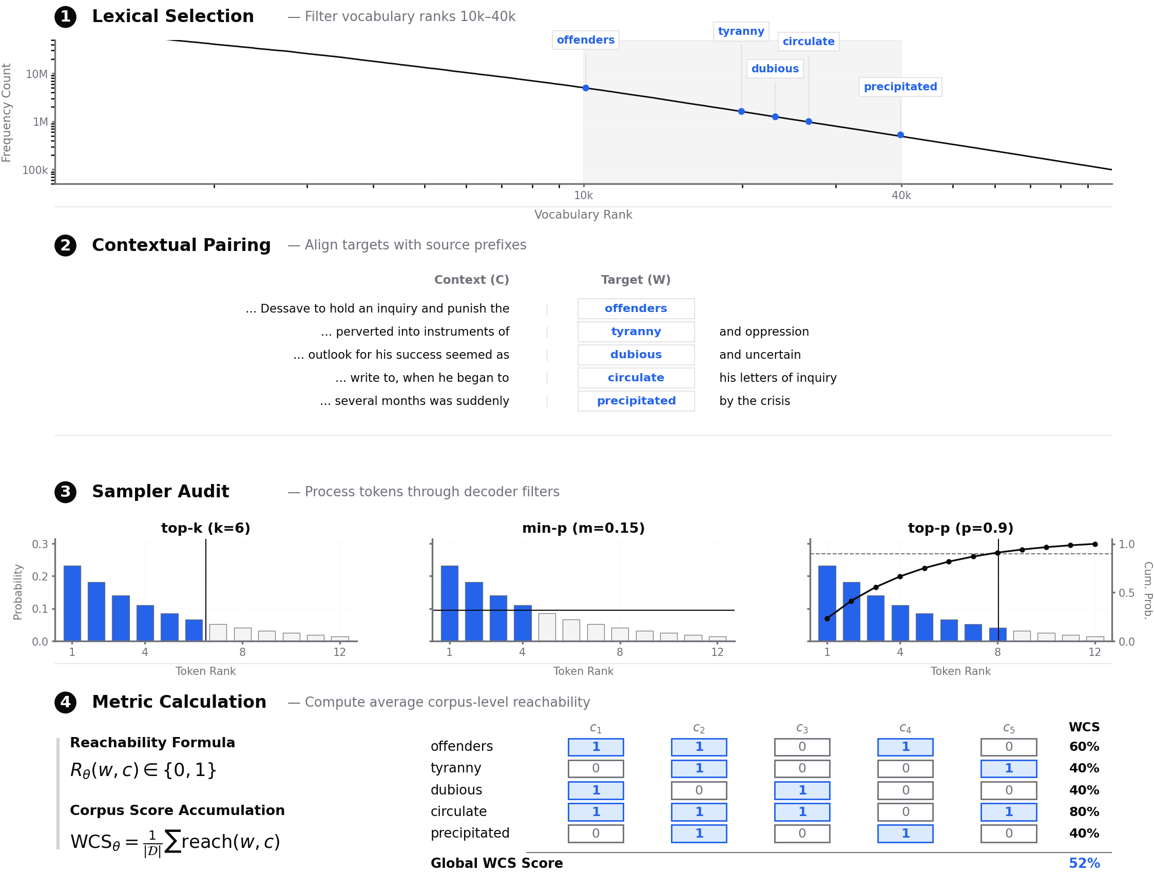
We recently released a preprint investigating whether common sampler settings filter out relatively common English words, rendering them impossible for LLMs to generate. We began by defining a frequency range of 10k to 40k on a word frequency list. These words are common enough that a human author uses them naturally. Examples closer to the 10k rank include poison, ethnicity, tourists, fatigue, coil, and consuming. On the rarer end, approaching the 40k rank, examples include instinctively, stiletto, eventful, lobsters, moustache, coals, and succulent. We randomly selected 100 words from this range; the full list is available here.
We searched for these words within PG19, a large corpus of human-authored texts. For each word, we extracted its surrounding context and verified with an LLM that the word makes sense in that context. This accounts for OCR or printing errors, and was necessary to automate because we looked at 1,000 contexts.
We then tested the logits assigned to each target word in its context across multiple open-weights LLMs. Using this data, we calculated whether the word would survive the initial selection phase under various sampler settings to remain a viable output option. We defined this using a binary reachability formula R θ(w, c) ∈ {0, 1}, which we aggregated into a Word Coverage Score across the corpus:
θ= 1 |D| Σ reach(w, c)
When sampler constraints are drastically loosened, allowing more tokens to survive sampling filters, most models predicted the majority of the words in at least one context. This confirms the models possess the vocabulary and are capable of producing the target word in the human context.
However, at recommended settings, every model tested failed to predict some of the words across all contexts, meaning that some words were not accessible in any tested context for certain models at the default settings. The percentage of words not predicted a single time at default settings ranged from 20% to 45%; interactive visualizers of these results can be viewed here.
We also evaluated the impact of temperature (T). Under top-p sampling, raising T from 0.7 to 1.0 yielded a significant increase in WCS, with diminishing returns as T approached 1.5. Because top-k sampling is purely rank-order based, the set of tokens it filters is entirely unaffected by temperature. Min-p proved less sensitive to temperature scaling than top-p; scaling T from 0.7 to 1.5 was required to increase the WCS for Llama-3.1-8B from 32.8% to 57.2%, whereas top-p achieves similar absolute gains merely scaling from 0.7 to 1.0.
We believe that with our paper we’ve introduced a way to quantitatively measure the effect of sampler settings on lexical diversity. As LLMs write more of the words we read, it’s important that we don’t lose the nuances and breadth of the language over time based on LLM influence. The effect of this is already visible and measurable, with the popularity of certain words in academic publishing rising and dropping with LLM trends; see Geng & Trotta, 2025.
At GING we research the limits and capabilities of LLMs, the applications of AI in science, research, psycholinguistics, and education. If you’re looking for collaborators or have ideas you want to discuss, feel free to reach out.
If you’re interested in whatever we publish next or my thoughts on AI, languages, and language learning, you can sign up for the mailing list or follow via RSS.
Stay in the loop #
Get new posts delivered to your inbox, or follow via RSS.
Update: Since writing this post, we’ve rerun the audit using a new corpus, FineWeb, and expanded it to 200 words with 50 contexts each. We also had the models write full-paragraph continuations after the human-written contexts, then correlated the lexical diversity of those continuations with the Word Coverage Score. The results show that a higher WCS predicts greater lexical diversity in LLM-generated text.