I work on security detection at Datadog. The model I have been building, Mambark, reads audit logs the way a language model reads text and scores every event by how surprising it is. It is a small model by today's standards, about 97 million parameters, and it looks at hundreds of billions of security events instead of sentences.
Generative models get talked about as machines for producing things. The claim of this post is that the same models, with nothing added and nothing fine-tuned, are also the most general anomaly detectors anyone has built, and that this is already changing how detection is done at scale. The mechanism turns out to be the very thing that makes them write.
The idea underneath is old and almost embarrassingly simple. I wanted to see it on its own, away from security telemetry and away from anything I cannot publish, so I built a small open-source project that runs it on plain English text. This post is what it shows.
Surprise is a score #
Any model that predicts what comes next is already an anomaly detector.
Hand it a prefix. It gives you a distribution over the next symbol. Now look at what actually came next and read off the probability it assigned. If the model said 0.4, nothing happened. If it said 0.0001, something happened.
Take the negative log and you have a number:
s_i = -\log P\!\left(x_i \mid x_1, \ldots, x_{i-1}\right)
That is the anomaly score. It is measured in nats, it is never negative, and it adds up: the surprise of a whole window is the sum of the surprises of its symbols, which is exactly the negative log-likelihood of that window. No labels, no list of known attacks, no rule describing what bad looks like. The only ingredient is a model of what usually comes next.
That distribution is worth looking at directly, because it is the same machinery that makes these models write:
One forward pass over the prefix produces one distribution over the entire vocabulary, 248,320 tokens for this model. To generate, you sample a token from that distribution, append it, and run the pass again. To score, you skip the sampling and instead look up the token that actually came next, then take minus log of the probability sitting in that slot. Same pass, same distribution, two different questions asked of it. Detection is generation with the sampling step replaced by a lookup.
The three panels are real output at three points in the contaminated text used later in this post. In ordinary English, after computer science that develops
, the model's favourites are algorithms
at 30.6% and intelligent
at 18.5%; the text said and
, its fourth choice at 6.8%, which costs 2.69 nats. Nothing happened. At the splice, after achieving defined goals.
, it expects a paragraph break or AI
or The
; it gets E
, ranked 602nd out of 248,320, probability 0.002%, and the score jumps to 11.09 nats. Something happened.
The third panel is the one I did not expect. By the end of the Basque sentence the model's third most likely continuation is E
at 10.4%, with Ez
and B
further down the list. It is expecting more Basque. It has moved its own notion of normal, in about two hundred characters, with no fitting and no retraining, and you can read that shift straight off the distribution.
None of that is specific to Qwen, or to language. Any model that puts a probability on the next symbol can be read this way. So the interesting question is not whether to score by surprise, it is which model you ask, because whatever you pick is what defines "usually" and therefore what counts as an anomaly.
Two ways to know what comes next #
A frequency table
The oldest answer is to count. A character n-gram model estimates P(c \mid \text{previous } n-1 \text{ characters})
by counting how often each continuation followed each context in some training text. To score a new character, you look up its context and read off the frequency. The model in this post is a 5-gram with interpolated smoothing, so it mixes the order-5 estimate with order-4, order-3, order-2, the unigram and a uniform term. Nothing ever gets probability zero, including characters it has never seen.
It is cheap, transparent and you can read the whole thing. It also has two properties that turn out to matter a lot.
You have to fit it, on the specific kind of text you are willing to call normal. And its memory is four characters. Everything before that is gone. A 5-gram deciding what comes after atio
does not know the text is in English, does not know it is about machine learning, and does not know that the same abbreviation appeared three hundred characters ago.
A pretrained sequence model
A language model conditions on the entire prefix. Every character since the beginning of the sequence is in the context window. And there is no fitting step: pretraining already covered English, French, Basque and Wikipedia prose, along with most other things. The model I used here is Qwen3.5-0.8B-Base, the base variant rather than the chat one, because post-training skews the distribution and makes it a worse likelihood estimator.
The consequence is the interesting part. The baseline is not fitted in advance, it is assembled on the fly out of the beginning of the very sequence being scored. The first sentence tells the model this is English, this is encyclopedic register, this is about artificial intelligence. Everything after is judged against that. One model, any normal.
The UEBA market runs on the first option
This is not an abstract distinction. It is the shape of a whole product category.
Exabeam's documentation is refreshingly direct about how its behavioral analytics works. "Our anomaly detection relies on statistical profiling of network entity behavior." "The statistical profiling is histogram frequency based." "Probability distributions are modeled using histograms." There are three model types: categorical, which "models a string with significance: number, host name, username", numerical clustered, and numerical time-of-week. Models are declared in a config file with a feature, a scope, an aging window and a convergence filter such as confidence_factor>=0.8
.
Read that as an n-gram and the mapping is exact. The feature is the context. The histogram over its values is the frequency table. The scope decides which normal you are fitting: this user, this peer group, the whole organisation. The convergence filter is the "have I seen enough to score yet" test. The aging window is refitting. Deployment guides commonly suggest thirty to sixty days of baselining before alerting goes live.
It works, and it has carried UEBA for a decade. But you pay both n-gram costs, per entity, forever. Every user, host and service needs its own fitted histogram for every feature you care about. A new employee has no baseline. A team that switches tools invalidates its baseline. And the context stays short by construction: a histogram of which hosts Alice signs into knows nothing about what Alice did in the previous ten minutes.
Which is why the complaint that follows UEBA around is always the same one: it is too noisy. Too many alerts that are merely unusual rather than wrong, and an analyst who stops reading them. Every mitigation the category has invented, convergence thresholds before a model is allowed to score, peer grouping, risk aggregation over many weak signals, exists to hold that floor down after the fact. Keep that complaint in mind, because the experiment reproduces it in miniature.
The newer generation takes the second option. Sweet Security aggregates events into sessions and has an LLM read the session, then labels each finding malicious, suspicious or bad practice. Mambark scores every event by negative log-likelihood under a model pretrained on next-event prediction. Different products, same move: replace the fitted per-entity table with a pretrained model of sequences in general.
An entity is a writer
Everything from here on is about English prose, so it is worth pinning down the mapping that makes it transferable.
An entity is a writer. A user, a host, a service account, an agent: each one emits a stream of events, and that stream is the text it writes. Each event is a token. What "normal" means for that writer is what normal means for prose, and it has the same three layers. A vocabulary: which APIs it calls, which hosts it reaches, which regions it appears in. A syntax: which event tends to follow which, in what order. And a register: bursty or steady, working hours or three in the morning, terse or verbose.
Under that mapping a UEBA histogram is a frequency table over one feature of one writer. It counts the letters Alice tends to use. It is a good count, and it will tell you when Alice uses a letter she has never used before, but it does not know what language she writes in or what she was saying a paragraph ago.
An anomaly is then a passage that does not read like the rest of the document. And the specific thing the experiment below is built around, a foreign sentence spliced into the middle of an English paragraph, is the case that matters most in security: somebody else started writing halfway through. Stolen credentials, a hijacked session, an insider stepping outside their role, an agent going off script. The document keeps Alice's name on it while the prose changes language mid-paragraph, and then changes back.
Read the figures that follow with that in mind. The English is Alice going about her week. The Basque sentence is somebody else at her keyboard. The French one is somebody else who has read her email and is trying to sound like her.
The experiment #
Everything below comes from one script in that project, which fetches its own data from Wikipedia so you can reproduce it.
The 5-gram is fitted on the English articles behind the searches "Machine learning", "Statistics", "Computer science" and "Mathematics". That is 193,003 characters, and it is deliberately generous: the same language and roughly the same subject as the text it will score.
The text being scored is the first 1,200 characters of the English article on artificial intelligence. It is not in the fitting corpus, but it could hardly be closer to it.
Then two contaminated copies, each with a single sentence spliced in after the first sentence. One is Basque, from the eu.wikipedia
article Euskara, the passage explaining that Basque is a language isolate. The other is French, from fr.wikipedia
's Langue basque, making the same point. They go into separate copies at the same position so both are measured against an identical background.
Qwen scores tokens, not characters, so each token's log-probability is divided by the number of characters it spans and shared out across them. That puts both models on the same axis.
Reading the figures
Every character is shaded by its surprise in nats, on one scale shared by every panel of every figure: 0.7 nats is left transparent, 7.7 nats and above is solid. Log-probabilities are comparable across models, a nat is a nat, so this is a fair side by side. Nothing is normalized per model and nothing is normalized per panel.
Under each panel the same numbers appear again as a trace, one point per character, from 0 to 8 nats, with the panel's own average as a dashed line. It is not smoothed. A moving average would be easier to threshold, but it would also spread the language model's boundary spikes into a plateau and destroy the thing worth looking at.
Clean text first #
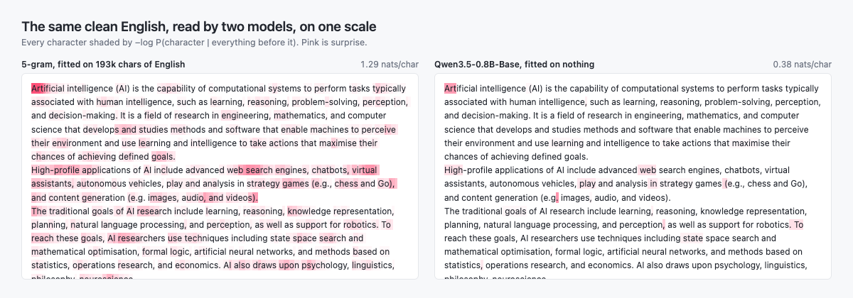
Start with text nobody has touched, read by both models:
The difference is hard to miss. After 193,003 characters of in-domain fitting, the 5-gram still spends 1.29 nats per character on ordinary English. Qwen spends 0.38, having been fitted on nothing at all. 4.5% of the n-gram's characters cost more than 3 nats, against 0.3% for Qwen. That is the noise floor, and it is what an analyst has to explain away before finding anything real. The arrows point at two of the loudest false alarms: 5.1 nats on web search
, 5.1 nats on virtual
. Both are plain English in an article about artificial intelligence.
The speckle is not random. Word beginnings cost the n-gram 1.64 nats against 1.27 inside a word, because four characters of context spanning a space carry almost nothing about which word starts next. Qwen has the same asymmetry but a milder one, 0.41 against 0.35. I expected word beginnings to dominate the n-gram's worst spikes and they do not: only 9 of its 50 most surprising characters are word-initial, the same count as Qwen. The systematic cost is real, the loudest alarms are elsewhere.
This is the UEBA critique, in one panel. 4.5% of characters past 3 nats is one flagged item in twenty-two, on a page where nothing whatsoever is wrong. Every one of them is a false positive, and web search
and virtual
are as loud as most of what the model will ever say. Put that same rate on a fleet of users and hosts, each with its own fitted histogram, and it is thousands of alerts a day to be looked at and dismissed. The noise is not a tuning failure that better thresholds would fix. It is what a short-context frequency table does when it meets ordinary variation it has not seen enough of. Qwen's floor on the same text is 0.3%, one in three hundred and thirty, with nothing tuned and nothing fitted.
The most surprising character on the whole clean page, for Qwen, is a full stop. The text writes (e.g., chess and Go)
early on and then (e.g. images, audio, and videos)
three hundred characters later. The second abbreviation ends without its comma, and that final dot costs 5.01 nats. It is Qwen's single worst character out of 1,200, and it is the one tall spike in an otherwise flat trace. The 5-gram scores the same character at 0.72 nats, which puts it in the least surprising quarter of the page. It is not that the n-gram disagrees. It cannot participate. The evidence sits three hundred characters outside its window.
That is the whole argument in one punctuation mark. Long context is not a nicety here. It is what lets a model be surprised by an inconsistency rather than by an unusual letter pair.
A Basque sentence #
Now splice one Basque sentence in after the first sentence and score the whole thing again:
Both models catch it, and the two signals do not look alike at all.
The n-gram lights the whole insertion and keeps it lit. Inside the spliced sentence it spends 5.27 nats per character against 1.31 outside, with 95% of the inserted characters past 3 nats. It never adapts, because it has nothing to adapt with. Basque is not in its table, from the first character to the last. It does not stop cleanly either. Nineteen characters after the splice ends it is still above its own average, and it reads 6.4 nats on the H
of High-profile
, which is plain English.
Qwen fires twice, once at each edge. The space before Euskara
costs 5.55 nats, the highest value it assigns anywhere in this text. Then it falls away fast: 2.15 on beste
, and by the end of the sentence izaten jarraitzen du
is running at 0.4 to 0.8 nats per character, ordinary-English territory. Within one sentence the model has rebuilt its baseline. This text is Basque now, and Basque is predictable. Then the sentence ends, English resumes, and it fires again: 2.07 nats on the line break, 2.19 on High
. Two spikes, one at each boundary, and very little in between.
Look at the two traces and the difference is the whole point. One is a raised plateau. The other is a flat line with a spike at the way in and a spike at the way out.
The two models are measuring different things. The n-gram reports a state, "this region does not match my table". Qwen reports a change, "something switched here, and switched back there". For an alerting pipeline the second is usually more useful, because it points at an event rather than at a region.
A French sentence #
Same background, same splice point, a French sentence this time:
French is the harder case, and it should be. It shares an alphabet, a lot of character statistics and a pile of vocabulary with English.
The n-gram degrades exactly as you would expect: 3.71 nats per character inside the insertion instead of 5.27, and 66% of the characters past 3 nats instead of 95%. The signal is still there, with less of it.
Qwen keeps the same two-spike shape. 5.62 nats at the boundary on C'est
, then a collapse. By typologique
at the end of the sentence it is down to 0.18 nats per character. Look at the phrase du point de vue
, which the inserted sentence happens to use twice: the second time round, point de vue
costs less than 0.01 nats per character. Effectively free. It is now both French and a repeat, and neither surprises the model any more.
Then English resumes and it fires again, 3.96 nats on the line break. That exit spike is nearly twice the Basque one. Same mechanism read backwards: the model had settled more completely into French than it ever did into Basque, so coming back out was more of a jolt.
Normal is whatever you fitted on #
One last control:
Same text, same model order, same code. The only change is the fitting corpus: this 5-gram was fitted on Basque Wikipedia instead of English.
The verdict inverts. It spends 4.31 nats per character on the English article and 1.45 on the Basque sentence, and 90% of the English characters pass 3 nats against 4.5% of the Basque ones. Those are the English-fitted model's own numbers with the roles swapped. The English is the anomaly now.
This is the control that makes the point unarguable. "Anomalous" is not a property of the text. It is a statement about the training distribution, and it is only as good as the match between that distribution and the thing you happen to be looking at. Every fitted baseline in every UEBA deployment carries this property. Fit on the wrong month, the wrong peer group or the wrong thirty days, and the model will confidently tell you the wrong text is foreign.
Being fair about it #
The LLM does not win on every axis, and the figures would be dishonest if I let you think it did.
Threshold each character on its own and count, and the n-gram marks far more of the insertion: 95% of the Basque characters pass 3 nats against Qwen's 3%. But counting flagged characters is the wrong question to ask of a signal shaped like Qwen's. It fires at both edges, and two edges are a region. The entry spike sits on the space before Euskara
, the exit spike on the newline that closes the sentence, and what lies between them is the insertion, delimited exactly. The n-gram's plateau is denser but blunter at the ends: nineteen characters after the splice is over it is still above its own average, reading 6.4 nats on the H
of High-profile
.
So the fair version of this is narrower. What a sustained signal buys is redundancy. The n-gram's evidence is spread over two hundred characters and no single one of them carries it. Qwen's sits in two tokens. Lose those, to a context window that truncates or a batch boundary that happens to fall there, and the region goes unmarked even though the model would have said so, loudly, at the moment it changed. Redundancy is worth something in a pipeline that drops data.
The catch is the floor everything sits on. The n-gram's loudest character on the clean page is 9.11 nats, on the A
of Artificial
, where it has no context yet. Nothing inside the Basque sentence gets that high; the worst there is 7.42. Its single biggest alarm on this page is a false one. Set the cold start aside and its worst clean character is 5.14 nats on web search
, with virtual
right behind at 5.08. Qwen's loudest character on the clean page is 5.01 nats, and that one is the e.g.
inconsistency, which is arguably a real find. Its loudest on the contaminated page is 5.55, at the splice.
Same units, same page. The n-gram is louder everywhere, including where nothing is wrong.
It also needed 193,003 characters of exactly the right sort of text to get there, and the mirror figure shows what happens when that assumption slips. Qwen needed nothing, and it spent 3.4 times less surprise on the clean page, which is 3.4 times less material to triage.
Fast rebaselining has a price too, and it is the same mechanism that makes it attractive. Qwen stopped being surprised by Basque after one sentence. An attacker who moves slowly enough becomes the new normal in exactly the same way. That is not a reason to avoid the approach, it is a thing to engineer: how long a context you score against, where you reset it, and whether a longer-horizon model runs alongside.
One last caveat. This is one text with two insertions, not a benchmark. Treat it as an illustration of a mechanism, not as evidence about which family of models is better.
What this looks like on security data #
Audit logs, authentication events, process trees, API calls: sequences of discrete events, produced by entities, with strong local structure and long-range dependencies. One writer per entity, one very long document each. Everything above transfers.
Mambark is what it looks like built for that. It is a Mamba selective state-space model of about 96.9 million parameters, started from the open mamba-130m
backbone, pretrained on next-event prediction over hundreds of billions of security events. State-space rather than transformer because the sequence lengths are brutal: a session can span thousands of events and a slow intrusion many more, and attention costs quadratic in that length while a state-space model costs linear. Events from every source are normalized the same way, grouped by entity, flattened into a fixed field structure and hashed into a shared vocabulary, so the architecture, tokenizer and training recipe stay identical across every benchmark with no hand-engineered features.
The scoring is exactly the formula at the top of this post.
The economics are why it is a small model. Running a frontier LLM over every event at enterprise scale would cost tens of millions of dollars a day. So Mambark is stage one of a retriever-reader pipeline: it scores everything in one forward pass and promotes around 10,000 candidates a day out of roughly 10 billion events, for tens of dollars of commodity GPU. Stage two hands that shortlist to an agent, which retrieves the user's recent activity, checks an asset's patch level, consults threat intelligence and writes up whether it is real. Also tens of dollars a day, and roughly four orders of magnitude cheaper than pointing the agent at the raw stream. Recall from the small model, precision and explanation from the agent.
On public benchmarks it reaches F1 1.000 on Thunderbird, 0.999 on BGL and 0.994 on UNSW-NB15, above the previous best, and trails slightly on LANL Cyber1 (AUC 0.987 against 0.990), HDFS (F1 0.941 against 0.980) and CERT Insider (AUC 0.879 against 0.910). The individual numbers matter less than the fact that one model with one recipe gets there on all of them. That is the property a per-entity histogram can never have.
Why this is a real break #
Detection engineering has spent twenty years encoding what somebody already knew to look for. There is a ladder in that, and each rung asks for less prior knowledge than the one below it.
A signature names the artifact: this file hash, this domain, this request string. It catches the attack it was written for and nothing adjacent to it. A correlation rule gives up the artifact and names the shape instead: twenty failed logins, then a success, then a new admin role, all inside five minutes. That survives a change of payload or tooling, but somebody still had to picture the sequence in advance and write it down. A fitted behavioral baseline gives up the picturing too. It learns what one entity normally does and flags departures from it, which is a real step, and still a narrow one: it knows a single entity, along the features you thought to model, and only once it has converged.
A pretrained sequence model encodes what usually happens. Not for this user, not for this feature, but in general. It can be surprised by something nobody wrote a rule for, in a place nobody thought to put a histogram, on an entity that has existed for four minutes. And the score it produces is a plain likelihood, which composes and thresholds like any other number.
Natural language processing took about a decade to make the jump from n-grams to pretrained models, and the jump did not make n-grams wrong. It made them the thing you reach for when you know exactly what you are modelling and you have the data to fit it. Security analytics is at the start of the same move, with the difference that the useful model is small and cheap enough to run on everything.
That is the part worth sitting with. The attention on generative AI goes to what it writes, but the same pretraining that makes a model fluent is what makes it a detector, and it arrives already knowing what normal looks like, for every entity, on day one. No fitting window, no per-user histogram, no thirty days of waiting. At the scale security data actually arrives at, that is not a better version of the old thing. It removes the step the old thing was built around.
The full report this post draws from, and the code that produces it, are at github.com/ngrislain/anomaly-detection. It is a small project, and more than half of it is the renderer for the figures above. Point it at your own text and see what surprises it.