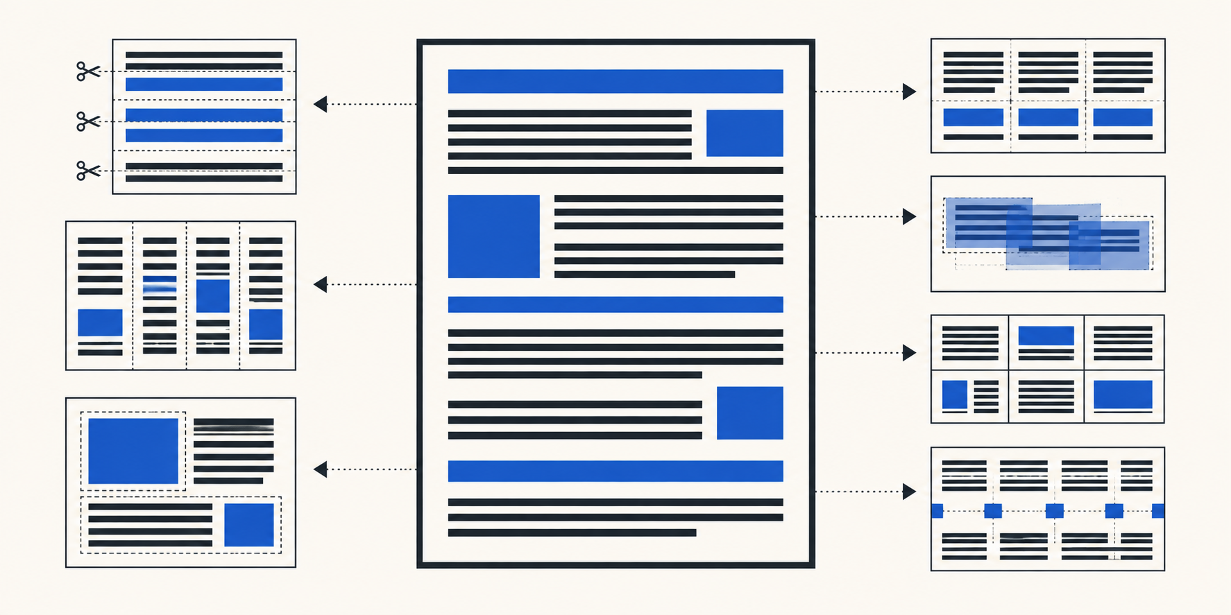
In this article, you will learn seven distinct chunking strategies for RAG pipelines, how each one works, and when to choose one over another for your specific use case.
Topics we will cover include:
- Why naive fixed-size token chunking destroys semantic meaning and how strategies like sentence-window retrieval and structural chunking preserve it.
- Advanced approaches including semantic chunking, hierarchical chunking, LLM-driven propositional chunking, and multi-modal table-preserving chunking.
- What matters beyond chunking strategy in production RAG systems, including index lifecycle management and chunk deduplication.
The Naive Approach Doesn’t Work #
Dumping unstructured text into a fixed-size token window and calling it a Retrieval-Augmented Generation (RAG) pipeline is a recipe for hallucination. RAG is essentially giving an AI an open-book test: the system searches a database for relevant notes, hands them to the large language model (LLM), and the model synthesizes an answer from those notes. But that database is entirely dependent on your chunking strategy — the rulebook used to slice a massive document into smaller pieces that an embedding model can read and store.
The naive approach of slicing documents into static 512-token arrays tears semantic boundaries in half, destroying context before the embedding model (the system that translates text into mathematical arrays) even sees it. Sever a negative qualifier from its subject, or split a function definition across two vectors, and the retriever is effectively blind, grabbing the wrong notes for the LLM’s open-book test.
One thing worth clarifying before we dig in: chunking (the deterministic or heuristic splitting of text strings) and parsing (extracting logical DOM/AST structures from raw document formats) are not the same thing. Bad parsing guarantees bad chunking, but even perfect parsing needs a solid chunking architecture to survive production query loads.
1. Fixed-Size Token Chunking with Overlap #
The Concept: Splitting text strictly by raw token counts using a sliding window to catch edge-boundary context.
How It Works: A fast tokenizer maps raw text to an integer array, slices it into uniform blocks (e.g. 512 tokens), and overlaps them by a fixed margin (e.g. 50 tokens) before decoding back to text strings for the embedding encoder.
Worth Noting: It’s structurally blind. You’ll inevitably slice a try/except
block down the middle or separate a pronoun from its antecedent. Overlap mitigates this slightly, but increases vector database bloat and ingestion compute costs linearly with the overlap ratio.
When to Use It: When processing homogenous, unstructured log files or flat text streams where structural boundaries don’t exist and ingestion latency is the top priority.
2. Sentence-Window Retrieval (Small-to-Big) #
The Concept: Embedding a granular chunk to maximize vector search precision, then returning the expanded surrounding context to the LLM during prompt assembly.
How It Works: At ingestion, documents are parsed into individual sentences. Each sentence is embedded and stored with a metadata pointer to its surrounding ( k ) sentences. At retrieval time, the vector database returns the top-( n ) nearest sentences, and the middleware swaps them out for their expanded text windows before hitting the generation model.
Worth Noting: Redundant context injection is a real risk here. If two adjacent sentences both clear the top-( k ) retrieval threshold, your middleware needs graph-based deduplication of the overlapping context windows. Skip that step, and you’ll blow out the LLM context window and trigger inference latency spikes.
When to Use It: When domain facts are densely packed and heavily nuanced (e.g. medical literature, legal statutes, etc.) where you need high retrieval precision without losing surrounding context.
3. Document-Aware Structural Chunking #
The Concept: Splitting documents along their logical markdown or DOM boundaries (H1, H2, paragraphs, list items) rather than arbitrary token limits.
How It Works: The pipeline uses parsers to build a tree of the document structure, chunks the leaf nodes (paragraphs and lists), and prepends the parent header hierarchy to each chunk (e.g., H1: Q3 Earnings > H2: Risk Factors > [Chunk]
). This preserves global context regardless of where the chunk ends up spatially.
Worth Noting: Node sizes are non-deterministic and vary widely. A large sub-section might still exceed your embedding model’s maximum sequence length (often 512 or 1024 tokens for dense encoders), forcing a fallback to token-based chunking, which risks breaking the structural integrity you just paid compute cycles to parse.
When to Use It: When ingesting heavily formatted corporate documents, API documentation, or contracts where the header hierarchy inherently defines the semantic payload.
4. Semantic (Embedding-Based) Chunking #
The Concept: Dynamically determining chunk boundaries by measuring the distance between sequential sentence vectors and splitting when semantic drift exceeds a threshold.
How It Works: Slide a sentence-level window across the text, generating lightweight embeddings for each sentence. Calculate the cosine similarity (mathematical closeness) between sentence ( i ) and ( i+1 ). If similarity drops below an empirically tuned hyperparameter ( \epsilon ), insert a hard chunk boundary. That drop signals a topic change.
Worth Noting: Ingestion latency and cost increase significantly. You’re forcing a forward pass through an encoder for every single sentence before you generate the final chunk embedding. And ( \epsilon ) is notoriously brittle — nearly impossible to tune globally across heterogeneous document sets.
When to Use It: When dealing with transcribed audio, meeting notes, or long-form narrative text that lacks structural formatting but contains distinct, unpredictable thematic shifts.
5. Hierarchical / Parent-Child Chunking #
The Concept: Creating a tree of chunks where multiple granular child nodes map to a single broad parent node. Retrieve enough children and you get the whole parent.
How It Works: Text is chunked at multiple granularities (e.g. 256 tokens and 1024 tokens). The 256-token chunks are embedded and mapped to their 1024-token parent via metadata foreign keys in the vector store. If ( >x% ) of a parent’s children are retrieved by the Approximate Nearest Neighbor (ANN) search, the query planner executes a merge and swaps the child chunks for the parent chunk.
Worth Noting: Managing the parent-child relational mapping in a distributed vector database gets complex fast. Deletes and document updates require cascading invalidations across the tree, and the merge logic at retrieval time adds latency to the critical path.
When to Use It: When query scope is highly variable — ranging from pinpoint factoid extraction to broad summarization of entire document sections.
6. Agentic (LLM-Driven) Propositional Chunking #
The Concept: Using an instruction-tuned LLM to read a text stream and inject structural breakpoints based on contextual understanding, or to extract atomic propositions.
How It Works: A document is streamed to a fast LLM with a strict system prompt instructing it to output a JSON array of natural breakpoints or distinct factual propositions. The ingestion pipeline then slices the raw document along those synthesized boundaries and embeds the extracted propositions.
Worth Noting: This guarantees non-deterministic ingestion. The LLM will hallucinate breakpoints, output malformed JSON, or silently drop text during extraction — any of which causes irrecoverable data loss in the index. It’s also significantly slower than programmatic chunking.
When to Use It: For highly valuable, irregular datasets where chunk quality drives the entire product’s viability, but only when ingestion runs in an asynchronous batch queue rather than a real-time stream.
7. Multi-Modal and Table-Preserving Chunking #
The Concept: Isolating tables, charts, and figures from standard text, extracting them as distinct objects, summarizing them for vectorization, and maintaining pointers back to the raw tabular data.
How It Works: A deterministic layout parser or Vision-Language Model (VLM) identifies a table. The pipeline extracts the raw HTML/Markdown, uses an LLM to generate a dense text summary of the table’s semantic insights, and embeds only the summary. The retrieval layer fetches the summary via ANN search but passes the raw Markdown table to the final generation prompt.
Worth Noting: If a table relies on surrounding text to make sense (e.g. “Results shown in Table 1 below normalized against the control group”), isolating it strips away necessary grounding and creates phantom references. Wide table schemas can also exceed the maximum sequence lengths of older generation models.
When to Use It: When ingesting financial reports, scientific papers, or heavily quantitative documents where standard recursive text tokenizers destroy spatial column alignment.
Looking Beyond Chunking #
Day 100 in production isn’t really about chunking strategies anymore. It’s about index lifecycle management, state synchronization, and pruning stale data. Document updates will inevitably create fragmented, orphaned chunks in your database. If you’re not implementing deterministic UUIDs based on cryptographic content hashes for your chunks and enforcing strict Time-To-Live (TTL) policies, your vector database will bloat with outdated text blocks. That leads to duplicate context injection at retrieval time, which silently degrades the LLM’s reasoning and inflates your token costs.
Stop obsessing over benchmark scores for the newest embedding model if your chunking strategy is an afterthought. The most capable dense retriever in the world can’t recover semantic meaning that was already mangled by a naive ingestion pipeline. Treat chunking as a foundational data modeling problem, test your boundaries aggressively, and build your system expecting structural failure.